1. Calibration workflow for nonlinear FEA
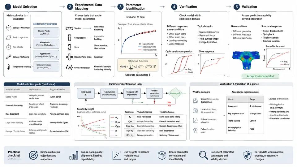
Nonlinear finite element analysis is only as trustworthy as the constitutive model driving it. A mesh can be refined, a solver can converge, and a contact algorithm can be tuned, yet the predicted response will still be wrong if the material model and its parameters do not represent the physical material under the actual loading path. Calibration is the disciplined process that closes this gap. It is not a single fitting exercise; it is a workflow with five interlocking stages: constitutive model selection, experimental data mapping, parameter identification, verification, and validation. Each stage has its own inputs, failure modes, and acceptance criteria, and skipping or reordering them is the most common reason calibrated models fail when transferred to a new component or load case.
Stage 1 — Constitutive Model Selection
Model selection starts from the physics of the problem, not from the software's default library. The engineer must first characterize the expected deformation regime and the dominant inelastic mechanisms. Relevant questions include: Are strains small (below roughly 5%) or large? Is the response rate-dependent? Is there a yield plateau, kinematic hardening under cyclic load, or hydrostatic-stress-sensitive behavior such as in polymers and soils? Does damage or failure need to be predicted, or only the pre-failure response?
For metals under monotonic loading with moderate strain, a von Mises yield surface with isotropic hardening (for example, a Swift or Voce hardening law) is often sufficient. If the component experiences load reversal or ratcheting, kinematic hardening (Armstrong–Frederick or Chaboche) becomes necessary because isotropic models cannot capture the Bauschinger effect. For rubber-like materials, hyperelastic models such as Neo-Hookean, Mooney–Rivlin, or Ogden are candidates, and the choice depends on the available test data and the strain range. Elastoplastic models with damage, such as Gurson–Tvergaard–Needleman or continuum damage mechanics formulations, are appropriate when void growth or stiffness degradation governs failure.
A practical rule: select the simplest model that captures the mechanisms active in the target application. Every additional internal variable adds parameters that must be identified from data, and poorly constrained parameters produce non-unique fits that may verify well on the calibration data but fail on validation.
Stage 2 — Experimental Data Mapping
Raw test data rarely maps directly onto model inputs. Mapping is the translation step: converting measured quantities into the stress–strain measures the constitutive model expects, at the correct reference configuration and under consistent sign and coordinate conventions.
Consider a uniaxial tension test on an aluminum alloy. The extensometer records engineering strain, and the load cell records force. To calibrate a finite-strain plasticity model, the engineer must convert engineering stress and strain to true stress and true strain using the incompressibility assumption in the plastic regime:
sigma_true = sigma_eng * (1 + e_eng)
eps_true   = ln(1 + e_eng)
where e_eng is engineering strain. This conversion is valid only up to the onset of necking; beyond that point, the stress state is no longer uniaxial and the data must be corrected or truncated. For a compression test, friction at the platens causes barreling, so the apparent flow stress is overestimated; the data may need a friction correction or the specimen must be re-tested with lubrication and a suitable aspect ratio.
Mapping also includes deciding which portion of the curve to use. The elastic modulus and Poisson's ratio are typically extracted from the initial linear region, while the hardening parameters are fitted to the plastic portion. Rate-dependent models require data at multiple strain rates, and cyclic models require stabilized hysteresis loops rather than the first cycle.
Stage 3 — Parameter Identification
Parameter identification is an optimization problem: find the parameter set that minimizes the discrepancy between model prediction and mapped experimental data. The objective function is usually a weighted sum of squared residuals:
J(p) = sum_i w_i * (sigma_model(eps_i; p) - sigma_exp_i)^2where p is the vector of material parameters and w_i are weights that reflect data reliability or normalize different test types. For a Voce hardening law, sigma_y = sigma_0 + Q*(1 - exp(-b*eps_p)), the parameters are the initial yield stress sigma_0, the saturation stress increment Q, and the saturation rate b. A typical identification for a 6061-T6 aluminum specimen might yield sigma_0 = 275 MPa, Q = 120 MPa, and b = 12, but these values are illustrative and must be replaced by actual fitted results for the specific material and heat treatment.
Identification is not just curve fitting. Parameters must be physically admissible: the elastic modulus must be positive, the hardening modulus must not be negative in a stable material, and the yield surface must remain convex. Constraints should be imposed during optimization. When multiple test types are available (tension, compression, shear), a simultaneous fit is preferred because it constrains the parameters more tightly and reveals whether a single parameter set can represent all loading modes.
Stage 4 — Verification
Verification answers the question: "Did I solve the equations correctly?" It is a numerical and mathematical check, not a physical one. Verification activities include:
- Confirming that the constitutive integration algorithm (for example, a return-mapping scheme for plasticity) converges and satisfies the consistency condition.
- Running a single-element test to compare the FEA response against the analytical stress–strain curve used for calibration.
- Checking mesh convergence for the calibration specimen model to ensure the extracted response is not mesh-dependent.
- Verifying that the implementation reproduces known limits, such as elastic behavior when the plastic strain is zero.
If the single-element simulation does not reproduce the calibration curve, the problem is in the implementation, the integration scheme, or the input mapping — not in the material physics. Verification must pass before validation is attempted.
Stage 5 — Validation
Validation answers a different question: "Did I solve the right equations?" It compares model predictions against independent experimental data that were not used during calibration. A validated model should predict the response of a different specimen geometry, a different loading path, or a different strain rate within an acceptable tolerance.
For example, if the model was calibrated on uniaxial tension, validation might use a notched tensile specimen, a shear test, or a cyclic loading test. The acceptance criterion should be defined before running the validation simulation — for instance, peak load within 5% and displacement at peak load within 10%. If the model fails validation, the engineer must return to model selection or data mapping, not simply add more parameters.
Closing the Loop
The five stages form a loop, not a line. Validation failures feed back to model selection or data mapping. Verification failures feed back to the integration algorithm or the mapping step. Parameter identification may need to be repeated with additional constraints if the fitted parameters are non-unique. The workflow is complete only when the model passes verification and validation against independent data, with documented acceptance criteria and parameter uncertainty.
A practical checklist for the calibration workflow:
| Stage | Key Question | Evidence of Completion |
|---|---|---|
| Model Selection | Does the model capture the active physics? | Documented justification with mechanism list |
| Data Mapping | Are the data in the correct stress/strain measure? | Converted curves with assumptions stated |
| Identification | Are parameters unique and physically admissible? | Residual plot, sensitivity, confidence intervals |
| Verification | Does the implementation reproduce the calibration curve? | Single-element comparison within tolerance |
| Validation | Does the model predict independent data? | Pass/fail against pre-defined criteria |
When this workflow is followed, the calibrated constitutive model becomes a defensible engineering asset rather than a curve-fit artifact. The next chapters will examine each stage in detail, beginning with the mechanics of model selection and the mathematical structure of common constitutive laws.