1. Nonlinear FEA landscape for large deform
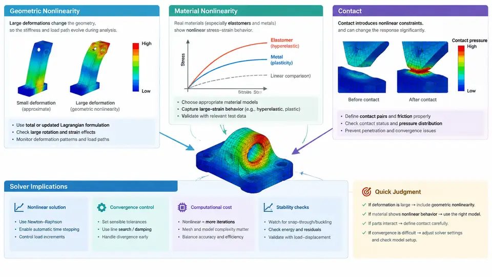
Large-deformation analysis is not a single switch that you flip on in a solver. It is a set of coupled physical effects — geometric nonlinearity, material nonlinearity, and contact — each of which changes the mathematical structure of the problem and, in turn, the numerical strategy required to solve it. This chapter maps that landscape so that later chapters on hyperelasticity, plasticity, and contact stabilization have a clear frame of reference.
Why "Large Deformation" Is a Different Problem
In linear FEA, the stiffness matrix K is assembled once, and the equilibrium equation K·u = F is solved in a single pass. This works because two assumptions hold: strains are small enough that the strain-displacement relationship is linear, and the material response is linear elastic. For elastomers stretched to 200–500% strain, or metal components that undergo plastic folding, both assumptions fail.
Geometric nonlinearity arises when the displacement field is large enough that the strain measure must include second-order terms. The Green-Lagrange strain tensor, for example, retains quadratic terms in the displacement gradient. This means the internal force vector becomes a nonlinear function of displacement, and equilibrium must be found iteratively — typically via Newton-Raphson, where each iteration solves K_T·Δu = R using the tangent stiffness K_T and the residual R = F_ext − F_int.
Material nonlinearity is independent of geometry. An elastomer's stress-strain curve is nonlinear and often nearly incompressible (bulk modulus ~1000× shear modulus), while a metal beyond yield follows a plastic flow rule with hardening. Both require the constitutive model to return not just stress but also the consistent tangent modulus, which feeds directly into K_T.
Contact nonlinearity adds a third layer: the active contact set changes as bodies deform, so the stiffness matrix itself changes topology between iterations. A node may be open in one iteration and closed in the next, introducing a step change in stiffness that can destabilize convergence.
How the Three Nonlinearities Interact
These effects are not additive — they compound. Consider a rubber seal compressed between two metal flanges. The elastomer undergoes large strain (geometric), its hyperelastic constitutive law is nonlinear (material), and the contact area with the flange grows as the seal bulges (contact). A solver that handles only one or two of these will either diverge or produce misleading results.
The practical consequence is that the tangent stiffness K_T must simultaneously account for:
- the geometric stiffness contribution from the current stress state (initial stress stiffness),
- the material tangent from the constitutive model at the current strain,
- the contact stiffness from the current active contact set and penetration state.
If any of these is inconsistent with the actual residual, Newton-Raphson loses its quadratic convergence rate and may stall entirely.
Solver Implications: What Changes in Practice
The most immediate practical consequence is that the load must be applied incrementally. A single-step load application that works for linear analysis will almost certainly diverge for large-deformation problems. The standard approach is a load-step / time-step scheme where each increment is solved to equilibrium before the next is applied.
Within each increment, the Newton-Raphson loop iterates until the residual norm falls below a tolerance. For well-behaved problems with consistent tangents, convergence is quadratic — typically 3–5 iterations. When the tangent is inconsistent or the problem is highly nonlinear, convergence degrades to linear or stalls.
Elastomers present a specific challenge: near-incompressibility causes volumetric locking in displacement-based formulations. The standard remedy is a mixed formulation (u/p) or selective reduced integration, both of which change the element formulation and the solver's degree-of-freedom count. Metals present a different challenge: plasticity introduces a yield surface that must be integrated at each Gauss point, and the return-mapping algorithm must produce a consistent tangent to preserve quadratic convergence.
Contact adds the most severe convergence difficulty. The active set changes discretely, so the residual is not smooth. Common stabilization strategies include:
- Penalty method: allows small penetration, adds contact stiffness proportional to a penalty parameter. Simple but sensitive to penalty value.
- Lagrange multiplier method: enforces zero penetration exactly, but adds DOFs and can produce zero diagonal terms.
- Augmented Lagrangian: combines both, iterating on penalty and multiplier to reduce penetration without ill-conditioning.
Choosing the Right Strategy
The table below summarizes how the dominant nonlinearity in a given problem shapes the solver configuration. This is not a rigid prescription but a starting point for the decisions that later chapters will detail.
| Dominant Nonlinearity | Typical Material | Key Solver Setting | Primary Risk |
|---|---|---|---|
| Geometric only | Metal, small plastic strain | NLGEOM on, automatic load stepping | Buckling / snap-through |
| Material only | Elastomer, moderate strain | Hyperelastic model, mixed u/p element | Volumetric locking, divergence at high strain |
| Contact dominant | Seal, gasket, impact | Augmented Lagrangian, contact stabilization | Chattering active set, rigid body motion |
| All three coupled | Rubber-metal bushing | Combined settings + line search | Slow or failed convergence |
What to Watch During a Run
Convergence behavior is diagnostic. A residual that decreases monotonically but slowly suggests an inconsistent tangent or a poorly conditioned system. A residual that oscillates suggests contact chattering or a limit point. A residual that grows indicates that the load increment is too large or the tangent is wrong.
For elastomers, also monitor the volume ratio J = det(F). If J deviates significantly from 1.0 in a nearly incompressible material, the element formulation is likely locking. For metals, monitor the equivalent plastic strain to ensure it remains within the calibrated range of the hardening curve. For contact, monitor the maximum penetration and the number of active contact points — a sudden jump in either often precedes divergence.
The next chapters will take each of these nonlinearities in turn, starting with the kinematic foundations of geometric nonlinearity and the strain measures that make large-deformation analysis mathematically consistent.