📚 Course ContentsChapter 1 Course overview

1. Course overview

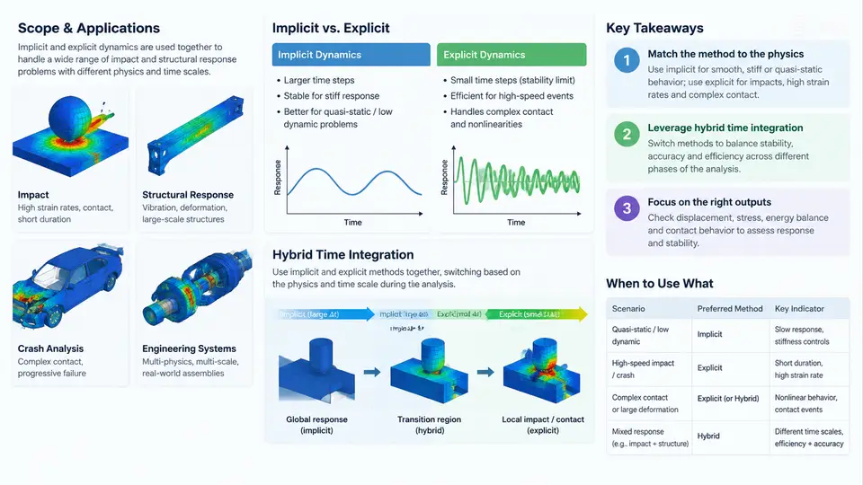
Structural dynamics problems differ less in their physics than in the time scales and nonlinearities they contain. A car body striking a rigid barrier, a fan blade ingesting a bird, a pressure vessel surviving a blast wave, and a printed circuit board enduring a drop test all share the same governing equation of motion, yet they demand very different numerical treatment. This chapter establishes the vocabulary and the decision framework that the rest of the course builds on: what implicit and explicit time integration actually do, where each is appropriate, and why production analyses of impact and structural response increasingly rely on hybrid schemes that combine both within a single run.

The governing equation and what "implicit" versus "explicit" really means

Every transient structural problem discretized by finite elements reduces to the semi-discrete equation of motion:

M · ü(t) + C · u̇(t) + F_int(u, u̇) = F_ext(t)

where M is the mass matrix, C the damping matrix, F_int the internal nodal force vector (a nonlinear function of displacement u and velocity u̇ once material and geometric nonlinearity are present), and F_ext the applied external load. The distinction between implicit and explicit integration lies entirely in how this equation is advanced from time step n to n+1.

Implicit methods (Newmark-β, HHT-α, generalized-α) evaluate equilibrium at the end of the step. Because F_int at time t_n+1 depends on the unknown u_n+1, a system of nonlinear algebraic equations must be solved, typically by Newton–Raphson iteration requiring the tangent stiffness matrix K_T = ∂F_int/∂u and repeated sparse linear solves. The payoff is unconditional stability for linear problems: the time step is chosen by accuracy, not by a stability ceiling.

Explicit methods (central difference, the basis of most commercial explicit codes) evaluate F_int at the known configuration t_n. No matrix factorization and no iteration are needed — the update is a vector operation. The price is conditional stability: the step must satisfy the Courant–Friedrichs–Lewy condition, approximately

Δt ≤ Δt_crit ≈ 2 / ω_max = L_e / c_d

where ω_max is the highest natural frequency of the mesh, L_e the smallest element characteristic length, and c_d the dilatational wave speed. For steel (E ≈ 210 GPa, ρ ≈ 7850 kg/m³), c_d ≈ 5170 m/s; a 2 mm element therefore imposes Δt_crit ≈ 0.39 µs. This single number explains most of the practical divide between the two families.

Where each method wins

Implicit dynamics dominates when the response is dominated by low-frequency structural modes and the loading is quasi-static or mildly dynamic: seismic response of buildings, modal superposition, rotor dynamics, and most linear or mildly nonlinear vibration work. A 1 s event with a 5 ms accuracy-driven step needs only 200 steps, and unconditional stability means mesh refinement does not shrink the step.

Explicit dynamics dominates when the physics itself is wave-dominated and highly nonlinear: crashworthiness, ballistic penetration, blast loading, drop tests, metal forming, and contact-intensive assembly. Here the time step is already forced to microseconds by wave propagation, so the stability limit costs nothing extra, and the absence of tangent stiffness and convergence iterations makes each step cheap and robust even when elements distort severely, materials fail, and contact status changes thousands of times per millisecond.

Rule of thumb: if the event duration is comparable to the time it takes a stress wave to traverse the structure, explicit is usually the right default. If the structure responds in its first few global modes and the event lasts many wave transits, implicit is usually cheaper.

Why hybrid time integration exists

Real engineering models rarely sit cleanly on one side of that line. A full vehicle model contains a stiff, contact-heavy front structure that demands explicit treatment and a large, mostly linear rear body and interior that would be wasteful to integrate explicitly. Aero-engine containment analyses couple a short, violent explicit impact phase to a long, low-amplitude residual vibration phase. A buried pipeline under blast loading has a local nonlinear region and a distant elastic soil domain.

Hybrid time integration addresses this by partitioning the model — by domain, by time, or both — and applying the appropriate integrator to each part. Three patterns recur throughout this course:

Domain decomposition (spatial partitioning): the nonlinear/contact region is integrated explicitly while the remainder is integrated implicitly, with interface tractions exchanged each step or each coarse step.
Sequential staging (temporal partitioning): an explicit phase captures the impact and early response; its state is then transferred as initial conditions to an implicit phase that resolves long-term residual response at far larger steps.
Adaptive switching: a single solver monitors stability and accuracy indicators and switches integration operators on the fly, for example explicit during contact transients and implicit during quiet intervals.

The engineering motivation is straightforward. In a representative crash model with roughly 3 million elements, an explicit run at Δt = 0.5 µs over 120 ms requires about 240,000 steps. If 70% of the mesh is nearly linear and could be advanced implicitly at 50 µs, the effective step count for that portion drops by two orders of magnitude. The savings are real, but they come with new failure modes: interface stability, energy conservation across the handoff, and consistent treatment of contact and constraints at partition boundaries.

What this course covers

The remaining chapters move from theory to production practice. We will derive the stability limits and accuracy orders of the standard integrators, then examine how mass scaling, selective subcycling, and element quality control keep explicit steps economical. We will treat contact algorithms — penalty, kinematic, and mortar — because contact is the single largest source of both cost and instability in impact models. Material models for metals at high strain rate (Johnson–Cook, Zerilli–Armstrong), failure and erosion criteria, and hourglass control receive dedicated treatment. The hybrid portion of the course covers domain decomposition, interface coupling schemes, sequential explicit-to-implicit handoff, and energy auditing across the transition.

Throughout, we will use a consistent sign and coordinate convention: displacements, velocities, and accelerations are positive in the global +X direction unless a local coordinate system is explicitly declared, and compressive stress is negative. Any figure or example that departs from this convention will state so at the point of use.

How to read the case studies: every worked example in this course states its geometry, material parameters, mesh size, time step, and boundary conditions explicitly. Where numbers are illustrative rather than measured, they are labelled as such. Your goal should be to reproduce the reasoning, not to memorize the numbers.

Key takeaways

Implicit and explicit integration solve the same equation of motion; they differ in where equilibrium is enforced and whether a linear solve is required.
Explicit stability is governed by Δt ≤ L_e / c_d; the smallest element and the stiffest material set the step for the entire model.
Implicit is preferred for low-frequency, long-duration, mildly nonlinear response; explicit is preferred for wave-dominated, contact-intensive, severely nonlinear events.
Hybrid schemes partition by domain, by time, or adaptively, and their principal engineering risks are interface stability and energy consistency at the handoff.
Correct interpretation of any dynamic result begins with the sign and coordinate convention, which must remain consistent between the model, the figures, and the reported quantities.