1. HPC-driven CAE simulation landscape
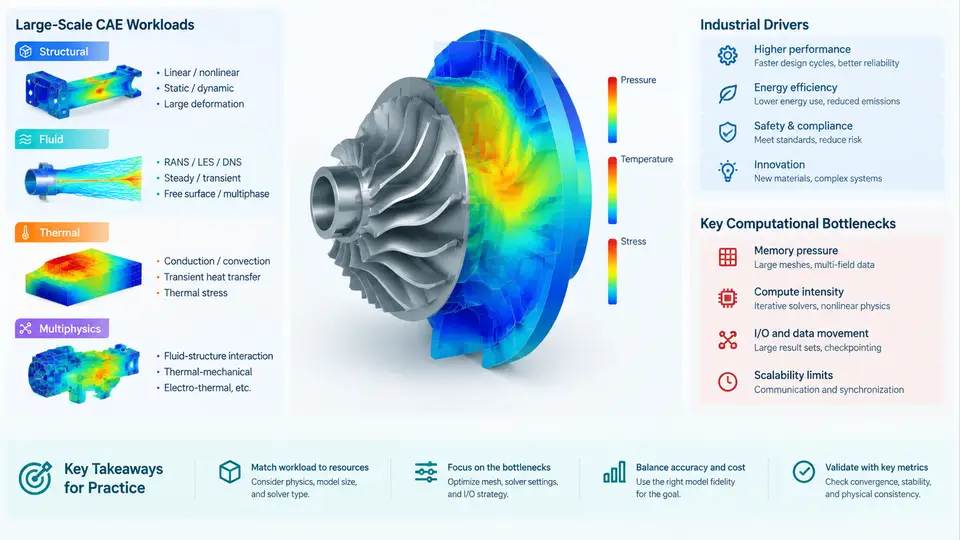
Computer-aided engineering (CAE) has shifted from a verification tool used at the end of a design cycle to a driver of design decisions. The reason is scale: modern simulation workloads routinely exceed what a single workstation can deliver in a useful turnaround time. High-performance computing (HPC) is what makes those workloads tractable. This chapter maps the landscape — the dominant workload classes, the industrial forces pushing them larger, and the computational bottlenecks that determine where time and money are actually spent.
Workload Classes and Their Computational Character
CAE workloads are not interchangeable. Each physics discipline stresses a different part of the compute/memory/communication balance, and that balance dictates how the workload must be parallelized.
Structural analysis (implicit FEA) solves a large sparse linear system K u = f at each load step. The dominant cost is sparse matrix factorization and iterative solution, which is memory-bandwidth-bound and scales poorly beyond a few thousand cores for a fixed problem size. Explicit dynamics (crash, impact) is different: it is compute-bound, embarrassingly parallel, and dominated by element-level stress updates with a stable time step governed by the Courant condition.
Computational fluid dynamics (CFD) solves the Navier–Stokes equations on meshes that may contain billions of cells. Pressure–velocity coupling (SIMPLE, PISO, or coupled algebraic multigrid) creates global dependencies that require frequent halo exchanges. CFD is typically communication-bound at scale, and the ratio of computation to communication per cell determines parallel efficiency.
Thermal analysis is often solved as a steady-state or transient conduction problem. It is comparatively cheap per degree of freedom but frequently coupled to structural or fluid solvers, which turns it into a multiphysics coordination problem rather than a raw throughput problem.
Multiphysics couples two or more of the above — conjugate heat transfer, fluid–structure interaction (FSI), aeroelasticity, or electromagnetics–thermal co-simulation. The coupling strategy (monolithic vs. partitioned, explicit vs. implicit) determines whether the bottleneck is solver time or inter-solver data exchange latency.
Industrial Drivers
Four industries dominate demand for large-scale CAE, and each pushes a different axis of the problem.
- Automotive: full-vehicle crash, NVH, and aerodynamics. Crash models with 20–50 million elements and hundreds of load cases create throughput pressure — many jobs, each needing to finish overnight.
- Aerospace: high-fidelity external aerodynamics, aeroelasticity, and certification loads. Mesh sizes of 109 cells and Reynolds-averaged or scale-resolving turbulence models push memory per node to its limit.
- Energy and turbomachinery: conjugate heat transfer in turbines, transient thermal cycling, and rotor dynamics. These are inherently multiphysics and require tight coupling between solvers.
- Electronics: thermal management of dense packages and drop/shock reliability. Many small-to-medium jobs with high parametric variation favor throughput-oriented scheduling over single-job scaling.
The common thread is that design space exploration — not a single simulation — is the real workload. A single high-fidelity run is a means; the goal is enough runs to make a decision. This is why HPC for CAE is as much a scheduling and data-management problem as a solver problem.
Computational Bottlenecks
Performance in large CAE is limited by four interacting constraints. Understanding which one binds a given job is the first step toward fixing it.
| Bottleneck | Typical symptom | Primary mitigation |
|---|---|---|
| Memory capacity | Job fails to allocate; must reduce mesh or increase nodes | Distributed-memory decomposition, out-of-core solvers, mesh coarsening |
| Memory bandwidth | Low FLOP/s per core; scaling flattens early | Cache blocking, higher arithmetic intensity, fewer cores per socket |
| Interconnect latency/bandwidth | Parallel efficiency drops sharply above ~1,000 ranks | Communication-avoiding algorithms, better partitioning, topology-aware mapping |
| Solver algorithmic scaling | Iteration count grows with problem size or core count | Multigrid preconditioners, domain decomposition with coarse-grid correction |
These are not independent. Adding nodes relieves memory capacity but increases communication; using more cores per node relieves interconnect pressure but worsens bandwidth contention. The practical skill is diagnosing which constraint is active before spending compute budget on the wrong fix.
Reading the Landscape: A Diagnostic View
The following diagram summarizes how a CAE workload moves from problem definition to a bottleneck diagnosis. It is not a workflow to follow step by step; it is a map of where the constraints live.
From Landscape to Practice
Before committing to a cluster run, a useful discipline is to estimate the binding constraint from problem size and hardware. Consider a concrete example: an implicit structural model with 30 million degrees of freedom, solved with a direct sparse solver. A rough rule of thumb for a 3D sparse factorization is that memory scales roughly as O(n^1.5) to O(n^2) depending on fill-in, while the factorization cost scales as O(n^2) to O(n^3). For n = 3×10^7, even the optimistic n^1.5 memory estimate is on the order of tens of terabytes — far beyond a single node. The practical response is either to switch to an iterative solver with a multigrid preconditioner, or to accept a domain-decomposition approach with a coarse-grid solve.
By contrast, an explicit crash model with the same element count is compute-bound and scales nearly linearly to thousands of cores, because each element update depends only on its immediate neighbors. The same "30 million" number therefore implies completely different HPC strategies. This is the central lesson of the landscape: problem size alone tells you almost nothing; the physics and the solver algorithm tell you everything.
What This Means for the Rest of the Course
The chapters that follow build on this map. Parallel decomposition strategies, solver selection, I/O and checkpointing, job scheduling, and performance profiling are all responses to the bottlenecks identified here. The goal is not to memorize the map but to develop the habit of asking, before every large run: which constraint is binding, and what is the cheapest way to relieve it?