1. FSI simulation engineering overview
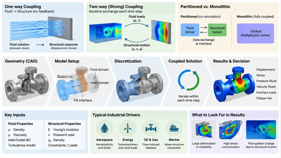
Fluid–structure interaction (FSI) simulation engineering is the discipline of predicting how a deformable or movable solid and a surrounding or internal fluid mutually influence each other, and then converting that prediction into an engineering decision. The defining feature of FSI is not simply that two physics are present, but that they are two-way coupled: the fluid pressure and shear stress load the structure, the structure deforms or moves, and that motion changes the flow domain and therefore the loads. When this feedback loop is neglected, the analysis degenerates into a one-way (uncoupled) problem, which is valid only when structural deformation is small enough that it does not measurably alter the flow field.
This chapter establishes the vocabulary, the coupling paradigms, the industrial motivations, and the end-to-end workflow that the remaining chapters build upon. The goal is to give you a mental model of where FSI sits in a simulation program and what decisions must be made before a single mesh is generated.
Coupling Paradigms
FSI problems are classified along two independent axes: how the two solvers exchange information in time, and how the interface conditions are enforced.
Monolithic (simultaneous) coupling assembles the fluid and structural equations into a single system and solves them together. It is numerically robust for strongly coupled problems such as large structural displacement in an incompressible flow, but it requires a unified solver and is expensive to develop and maintain.
Partitioned (staggered) coupling keeps separate fluid and structural solvers and exchanges interface data at synchronization points. This is the dominant industrial approach because it reuses mature, validated single-physics solvers. Within partitioned coupling, two time-integration schemes matter:
- Explicit (loosely coupled) scheme: solve fluid, transfer loads to the structure, solve structure, transfer displacement back, advance one time step. It is cheap per step but can diverge when the added-mass effect is strong (e.g., a light structure in a dense fluid).
- Implicit (strongly coupled) scheme: iterate within each time step until the interface residual (load and displacement) falls below a tolerance. It is stable for strong coupling but costs several fluid and structural solves per step.
Interface conditions are enforced either by a conforming mesh (shared nodes at the interface) or by non-conforming interpolation (load and displacement mapped between dissimilar meshes). Non-conforming mapping is almost always required in practice because fluid and structural meshes have different refinement requirements.
Industrial Drivers
FSI simulation is driven by failure modes and performance requirements that single-physics analysis cannot capture. Representative industrial drivers include:
| Industry | Representative FSI Problem | Engineering Consequence |
|---|---|---|
| Aerospace | Wing flutter, control-surface buzz | Aeroelastic instability, structural fatigue |
| Energy / Turbomachinery | Blade vibration in compressors and turbines | High-cycle fatigue, blade failure |
| Automotive | Fuel-tank sloshing, tire hydroplaning | Noise, handling loss, structural loads |
| Biomedical | Arterial wall deformation under pulsatile flow | Stent migration, aneurysm rupture risk |
| Civil / Offshore | Vortex-induced vibration of risers and cables | Fatigue damage, mooring failure |
In each case, the decision the simulation supports is concrete: change a geometry, adjust a material, add a stiffener, or set an operating limit. FSI simulation earns its cost when it replaces or reduces physical testing and when it explains a failure that single-physics analysis missed.
The Simulation Workflow from CAD to Decision
The workflow below is the backbone of this course. Each stage has a distinct deliverable and a distinct failure mode.
- CAD preparation and geometry simplification. Remove features that do not affect the physics (small fillets, bolt holes, logos), but retain features that control flow separation or structural stiffness. Deliverable: a clean, watertight geometry suitable for meshing.
- Domain decomposition and meshing. Build the fluid domain and the structural domain, and define the FSI interface. Decide on conforming or non-conforming interfaces. Deliverable: fluid mesh, structural mesh, and interface definition.
- Physics setup. Assign fluid properties (density, viscosity, compressibility), structural properties (elastic modulus, Poisson ratio, density), boundary conditions, and initial conditions. Deliverable: a fully specified case.
- Coupling configuration. Select monolithic or partitioned coupling, explicit or implicit time integration, under-relaxation factors, convergence tolerances, and time-step size. Deliverable: a coupling scheme with documented stability margins.
- Solve and monitor. Run the simulation while monitoring interface residuals, energy balance, and physical quantities of interest. Deliverable: a converged, physically consistent solution.
- Post-processing and verification. Extract displacements, stresses, pressures, frequencies, and compare against analytical benchmarks or experimental data. Deliverable: a verified result with quantified uncertainty.
- Decision. Translate the result into a design or operating decision, with a clear statement of assumptions and limitations. Deliverable: a decision record.
The following SVG illustrates the coupled data flow and the decision loop that connects these stages.
What Makes FSI Simulation Engineering Difficult
Three difficulties distinguish FSI from single-physics simulation and explain why a dedicated engineering discipline exists.
First, the interface is a moving boundary. The fluid mesh must deform or be remeshed as the structure moves. Poor mesh quality at the interface causes solver divergence or inaccurate loads. This is why dynamic-mesh or ALE (Arbitrary Lagrangian–Eulerian) formulations are central to FSI.
Second, the coupling can be numerically unstable. The added-mass instability, mentioned earlier, is the classic example. A practical symptom is that interface displacement grows without bound even though each individual solver reports convergence. The standard remedies are implicit coupling, under-relaxation (typical starting values 0.2–0.5 for strong coupling), or a Robin-type interface condition.
Third, verification is non-trivial. There is rarely an exact solution for a real FSI problem. Engineers rely on benchmark cases such as the Turek–Hron flag-and-cylinder benchmark, analytical limits (e.g., small-amplitude limit), grid and time-step convergence studies, and experimental validation.
From Simulation to Decision
The final stage is the one most often under-documented. A simulation result becomes a decision only when it is accompanied by a clear statement of the question being answered, the assumptions made, the quantified uncertainty, and the resulting recommendation. For example, a vortex-induced vibration study might conclude: "At the design current speed of 1.2 m/s, the riser's cross-flow response amplitude is 0.4D, which exceeds the fatigue limit of 0.3D; adding a helical strake reduces it to 0.15D." That statement is a decision, not a contour plot.
Throughout this course, every chapter will connect back to this workflow. The next chapters move into the governing equations and the mathematical formulation of the coupled problem, which provide the foundation for the numerical methods and engineering practices that follow.