1. Course overview
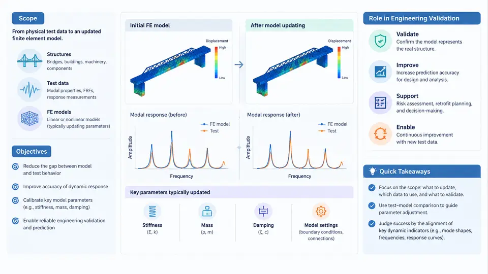
Finite element model updating is the systematic process of adjusting the parameters of a numerical model so that its predicted dynamic behavior matches measured behavior from a physical structure. In structural dynamics, the finite element (FE) model is rarely correct on the first attempt. Idealized joints, uncertain boundary conditions, unmodeled stiffness from non-structural elements, and material property scatter all introduce discrepancies between prediction and reality. Model updating closes that gap by treating the FE model as a parameterized hypothesis and the measured data as evidence.
This course addresses the full workflow: from planning a modal test and extracting clean experimental data, through sensitivity analysis and parameter selection, to solving the optimization problem and validating the updated model against independent data. The scope is deliberately practical. Every concept is tied to a concrete step that an engineer performs on a real structure — a beam, a plate, a frame, or a built-up assembly — using standard tools such as impact hammers, accelerometers, and commercial FE software.
Why Model Updating Matters
An unvalidated FE model can be dangerously misleading. A model that predicts a first bending frequency 15% higher than the measured value may still look plausible in a report, but it will misguide fatigue life estimates, vibration isolation design, and structural health monitoring thresholds. Model updating transforms the FE model from a nominal design artifact into a calibrated digital twin that reflects the as-built structure.
The role of model updating in engineering validation is threefold:
- Diagnosis: Identify which physical parameters (stiffness, mass, damping, boundary stiffness) are responsible for observed discrepancies.
- Correction: Adjust those parameters within physically meaningful bounds to minimize the error between predicted and measured modal properties.
- Confidence: Quantify the remaining uncertainty and demonstrate that the updated model generalizes to load cases or modes not used in the updating process.
The Updating Workflow at a Glance
Although every project differs in detail, the core sequence is consistent. The SVG below maps the data and parameter flow across the major stages, from physical test to validated model.
What You Will Be Able to Do
By the end of this course, you should be able to independently execute a model updating campaign on a laboratory or industrial structure. Specifically, you will be able to:
- Design a modal test that produces data suitable for updating — selecting excitation, sensor placement, and frequency bandwidth based on the modes of interest.
- Extract modal parameters from measured frequency response functions (FRFs) and assess their quality using coherence and stabilization diagrams.
- Pair experimental and analytical modes using the Modal Assurance Criterion (MAC) and identify which parameter sensitivities are high enough to be updated reliably.
- Formulate and solve the updating problem as a bounded least-squares or Bayesian inference problem, and interpret the resulting parameter changes physically.
- Validate the updated model against data not used in the updating, and report the remaining uncertainty honestly.
A Concrete Example: Updating a Cantilever Beam Model
Consider a steel cantilever beam, 500 mm long, 30 mm wide, and 5 mm thick. The initial FE model uses nominal values: Young's modulus E = 210 GPa, density ρ = 7850 kg/m³, and a perfectly fixed boundary at one end. A modal test with an impact hammer and a single accelerometer at the free tip yields the first three bending frequencies: 16.2 Hz, 101.5 Hz, and 284.0 Hz.
The initial FE model predicts 17.1 Hz, 107.2 Hz, and 300.1 Hz. The errors are +5.6%, +5.6%, and +5.7% — a consistent overprediction. This pattern suggests a global stiffness or mass discrepancy rather than a local joint issue. A sensitivity analysis shows that the first three frequencies are most sensitive to E and ρ, and relatively insensitive to the boundary stiffness once it exceeds 10⁶ N/m.
Selecting E and ρ as updating parameters, with bounds of ±10% around nominal, the optimization minimizes the weighted frequency error. The updated values are E = 198 GPa and ρ = 7920 kg/m³. The updated model predicts 16.3 Hz, 101.8 Hz, and 284.5 Hz — all within 0.6% of the measured values. A fourth mode at 520 Hz, not used in the updating, is predicted at 523 Hz, confirming that the update generalizes.
Common Pitfalls and How to Avoid Them
Model updating fails in predictable ways. Being aware of these failure modes early will save considerable time:
| Pitfall | Symptom | Mitigation |
|---|---|---|
| Updating too many parameters | Optimization converges to non-physical values; poor validation | Use sensitivity analysis to select only parameters with high influence and low correlation |
| Ignoring mode pairing errors | MAC values below 0.7; frequency errors inconsistent across modes | Verify mode pairing manually; check MAC matrix before updating |
| Over-reliance on a single mode | Updated model matches one mode but degrades others | Include multiple modes in the objective function with appropriate weighting |
| No independent validation | Updated model appears perfect but fails on new data | Reserve at least one mode or load case for validation only |
How This Course Is Organized
The course progresses from measurement fundamentals to advanced updating techniques. Early chapters cover experimental modal analysis, signal processing, and data quality assessment. The middle section develops the theoretical framework: correlation criteria, sensitivity analysis, regularization, and optimization algorithms. Later chapters address Bayesian updating, uncertainty quantification, and applications to real-world structures such as automotive bodies, aerospace panels, and civil infrastructure. Each chapter includes a hands-on component using representative data and open or commercial tools.
The goal is not to turn you into a software operator, but into an engineer who understands what the model is telling you, when to trust it, and when to question it. Model updating is a dialogue between simulation and experiment; this course teaches you how to conduct that dialogue rigorously.