1. Introduction to composite structures sim

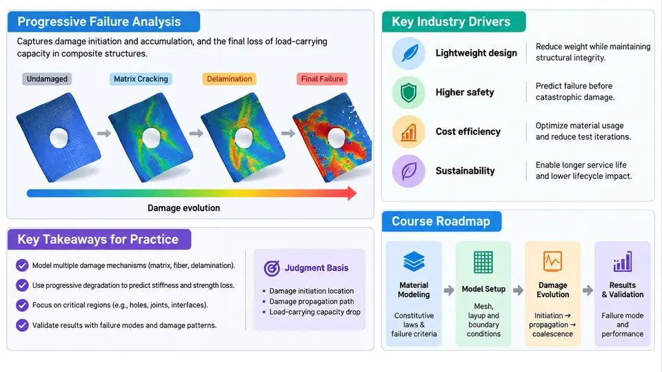
Composite materials have become the default structural solution wherever stiffness-to-weight and strength-to-weight ratios dominate design decisions: commercial airframes, wind turbine blades, Formula 1 monocoques, pressure vessels, and increasingly automotive body structures. Yet the same anisotropy and heterogeneity that make laminates so efficient also make them difficult to certify. A metallic component fails by crack initiation and propagation in a largely isotropic medium; a laminated composite accumulates damage — matrix microcracks, fiber–matrix debonding, delamination, and finally fiber fracture — often with little or no visible external indication. Capturing that accumulation numerically is the job of progressive failure analysis (PFA).

Why Progressive Failure Analysis Matters

Classical laminate theory and first-ply-failure (FPF) criteria such as Tsai–Hill or Tsai–Wu answer a single question: at what load does the first ply exceed its allowable? That is a conservative but often wasteful answer. Test coupons routinely carry 1.5–3× the FPF load before catastrophic rupture, because the first ply to fail is usually a transversely loaded 90° ply whose matrix cracks redistribute load to adjacent 0° plies. Designing to FPF therefore over-engineers the structure; designing to last-ply failure without tracking the intermediate damage state is unsafe, because the load path has changed and the residual stiffness is unknown.

PFA closes this gap by coupling a stress solver to a damage model that evolves. At each increment the solver computes ply-level stresses in the material coordinate system (1 = fiber, 2 = transverse, 3 = thickness), evaluates a failure criterion, degrades the stiffness of failed integration points according to a defined law, and re-equilibrates. The output is not a single number but a damage trajectory: stiffness degradation versus applied strain, the sequence of failure modes, and the ultimate collapse load.

Industry Drivers

Three forces push PFA from research into production workflows. First, certification credit: airworthiness authorities accept building-block test pyramids, and simulation that credibly predicts damage onset and growth can reduce the number of expensive full-scale tests. Second, weight reduction: if the post-FPF reserve is quantified rather than assumed, plies can be removed. Third, damage tolerance: impact and manufacturing defects (porosity, wrinkles, ply drops) must be assessed for residual strength, and only an evolving damage model can represent the interaction between an existing defect and subsequent loading.

The practical consequence is that the analyst must master three coupled domains: laminate mechanics (CLT, ply coordinates, failure criteria), damage mechanics (softening laws, fracture energies, regularization), and numerical implementation (explicit vs. implicit solvers, mesh objectivity, convergence).

Where PFA Sits in the Simulation Stack

The diagram below shows the analysis chain and the feedback loop that distinguishes PFA from a linear static run. The key structural feature is the return path from the failure evaluation back to the constitutive update — without it, the analysis is only FPF.

What the Course Covers

The 30 chapters follow a deliberate progression from theory to validated practice. The early block establishes laminate mechanics and failure criteria, because a PFA is only as good as the criterion feeding it. The middle block builds the damage model: continuum damage mechanics, smeared cracking, cohesive zone modeling for delamination, and the regularization techniques (viscosity, characteristic length, crack-band) that keep results mesh-objective. The later block applies the machinery to real problems — open-hole tension, low-velocity impact, compression after impact, bolted joints, and ply-drop regions — and closes with verification and validation against test data.

Throughout, the emphasis is on decisions an analyst actually makes: which criterion for which mode, how to set fracture energies from coupon data, how to choose element size relative to the cohesive zone length, when an explicit solver is preferable to implicit Newton–Raphson, and how to recognize a non-physical result (snap-back without regularization, damage spreading one element per increment, or a load–displacement curve that never softens).

A First Worked Example: Open-Hole Tension in a Quasi-Isotropic Laminate

Consider a 200 mm × 40 mm coupon with a 6 mm central hole, layup [0/45/−45/90]₂ₛ, 0.125 mm ply thickness (2 mm total), loaded in tension. Material properties representative of an intermediate-modulus carbon/epoxy: E1 = 135 GPa, E2 = 9.5 GPa, G12 = 5.0 GPa, ν12 = 0.30, Xt = 2100 MPa, Xc = 1400 MPa, Yt = 60 MPa, Yc = 220 MPa, S = 90 MPa. Fracture energies for the damage model: Gf = 90 N/mm (fiber), Gm = 0.6 N/mm (matrix).

A practical workflow proceeds as follows. Build a quarter-symmetric shell or solid model with a refined mesh near the hole; the element size near the stress concentration should be no larger than the cohesive zone length lc ≈ E2·Gm / (Yt²) ≈ 9.5e3 × 0.6 / 60² ≈ 1.6 mm, so a 0.5 mm seed is a reasonable starting point. Apply symmetry boundary conditions, fix one end, and drive the other end with displacement control at 0.5 mm per step — displacement control is preferred here because it captures the post-peak softening branch that load control cannot follow.

Expected observations, in order: matrix cracking initiates in the 90° plies at the hole edge at roughly 0.4–0.5% applied strain; the load–displacement curve shows a knee as those plies degrade; damage then spreads into the ±45° plies and delamination begins at the hole boundary; final fiber failure in the 0° plies occurs near 1.2–1.4% strain. The analyst should verify that the reaction force rises monotonically to a peak, then softens gradually — a sudden drop to zero indicates insufficient regularization or an over-coarse mesh.

How to Use This Course

Each chapter pairs the governing equations with a concrete modeling decision and, where useful, a reproducible example with stated inputs and observable outputs. Readers are encouraged to reproduce the open-hole example above in their own solver as a baseline, then perturb one parameter at a time — mesh size, fracture energy, criterion — and observe how the load–displacement curve responds. That habit of controlled perturbation is what separates an analyst who runs PFA from one who understands it.