1. Industrial data platform landscape
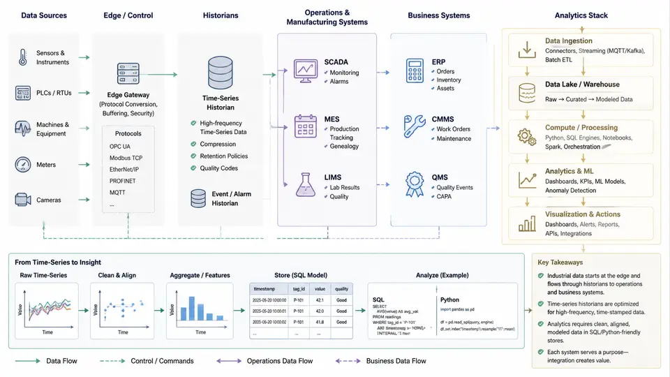
An industrial data platform is not a single product but a layered ecosystem that moves data from physical processes to analytical decisions. Understanding this landscape is the foundation for every SQL query and Python pipeline you will build in this course. The core challenge is that operational technology (OT) and information technology (IT) evolved separately, with different protocols, time semantics, and reliability requirements. A successful analytics stack must bridge that gap without losing fidelity or context.
The Five Data Domains
Industrial data originates from five broad domains, each with distinct characteristics:
- Sensors and actuators — raw analog and digital signals at the edge. A vibration sensor might sample at 25.6 kHz; a temperature transmitter might report every 500 ms via 4–20 mA or HART. These are high-frequency, low-context streams.
- SCADA (Supervisory Control and Data Acquisition) — the real-time control layer. SCADA systems poll PLCs and RTUs, maintain tag databases, and present HMI screens. Data here is current-value oriented, often with 1-second or sub-second scan rates.
- Historians — purpose-built time-series databases such as OSIsoft PI, Honeywell PHD, or open alternatives like TimescaleDB and InfluxDB. Historians store compressed, timestamped tag values with high write throughput and efficient range queries. They are the primary source for trend analysis and process analytics.
- MES (Manufacturing Execution Systems) — transactional systems that track work orders, batches, material genealogy, and quality results. MES data is event-driven and relational, often with complex state machines.
- ERP (Enterprise Resource Planning) — business-level systems (SAP, Oracle, Microsoft Dynamics) holding production orders, inventory, maintenance schedules, and cost data. ERP data is batch-oriented, with daily or shift-level granularity.
The analytics stack sits above these domains, typically comprising a data ingestion layer (OPC UA, MQTT, REST, JDBC), a storage layer (historian, data lake, relational warehouse), a transformation layer (SQL, Python, dbt), and a presentation layer (dashboards, notebooks, APIs).
Why the Boundaries Matter
The separation between OT and IT is not bureaucratic — it reflects real engineering constraints. OT systems prioritize determinism and availability: a SCADA scan must complete within its cycle time, and a historian must never drop a critical alarm event. IT systems prioritize consistency and flexibility: an ERP transaction must be ACID-compliant, and a data warehouse must support ad-hoc queries. When you write SQL against historian data, you are querying a system optimized for time-range retrieval, not for joins. When you join historian tags to MES work orders, you are crossing a semantic boundary: the historian knows what happened at a timestamp, while MES knows why it happened.
Practical Example: Correlating Vibration with Work Orders
Consider a real scenario: a pump on Line 3 shows rising vibration. The historian has tag LINE3.PUMP01.VIBRATION sampled at 1 Hz. MES has a work_orders table with equipment_id, start_time, end_time, and product_code. To find whether vibration spikes correlate with specific product runs, you would:
- Extract historian data for the shift window using a time-range query (e.g., PI SQL or TimescaleDB
time_bucket). - Aggregate to 1-minute averages to reduce noise and align with MES event granularity.
- Join on
equipment_idand timestamp overlap using a non-equi join or interval join. - Compare mean vibration per
product_codeand flag runs exceeding a threshold (e.g., 4.5 mm/s RMS).
A sample SQL fragment for the join might look like:
SELECT w.product_code,
       AVG(h.vibration) AS avg_vib,
       COUNT(*) AS samples
FROM historian_1min h
JOIN work_orders w
  ON h.equipment_id = w.equipment_id
 AND h.ts >= w.start_time
 AND h.ts <  w.end_time
WHERE h.ts BETWEEN '2025-03-01 06:00' AND '2025-03-01 14:00'
GROUP BY w.product_code
ORDER BY avg_vib DESC;
If the query returns a product code with avg_vib consistently above 4.5 mm/s while others remain below 2.0, that is a actionable signal — not proof of causation, but a prioritized lead for maintenance investigation. The key engineering discipline is to always validate timestamp alignment: historian timestamps are often in UTC, while MES may use local plant time. A one-hour offset can silently invalidate the entire analysis.
The Analytics Stack in Practice
A typical industrial analytics stack for this course uses:
| Layer | Typical Technology | Primary Role |
|---|---|---|
| Ingestion | OPC UA, MQTT, JDBC, REST | Move data from OT/IT sources |
| Storage | Historian, PostgreSQL, Parquet | Persist time-series and relational data |
| Transformation | SQL, Python, dbt | Clean, join, aggregate, feature-engineer |
| Presentation | Grafana, Power BI, FastAPI | Visualize and serve results |
Your role as an analytics engineer is to own the transformation layer: writing SQL that respects time-series semantics, using Python for statistical validation and anomaly detection, and ensuring that every join across domains is semantically correct. The next chapters will build these skills incrementally, starting with SQL fundamentals applied to historian-style data.
COUNT(*) does not equal elapsed time. Always use time-weighted averages or explicit resampling when calculating rates or durations.