1. Reliability engineering fundamentals
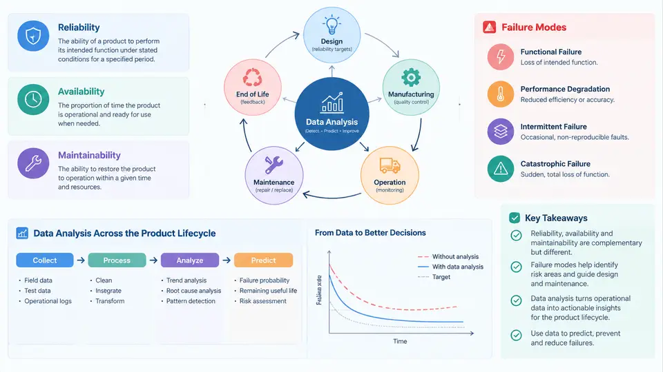
Reliability engineering is the discipline that quantifies how long a product will perform its intended function without failure, and then uses that quantification to drive design, manufacturing, and service decisions. In modern practice, reliability is not a post-design verification activity; it is a lifecycle discipline in which field data, test data, and design models continuously inform one another. This chapter establishes the vocabulary and the measurement framework that every later technique — Weibull analysis, accelerated life testing, FMEA, RCM, prognostics — depends on.
Core Definitions and Their Precise Meaning
Reliability is the probability that an item performs a required function under stated conditions for a stated period of time. Every word in that definition is load-bearing. "Probability" means reliability is a statistical statement, never a guarantee for a single unit. "Required function" means the function must be explicitly defined — a pump that delivers 80% of rated flow may be "failed" for one application and "operating" for another. "Stated conditions" covers load, temperature, humidity, duty cycle, and maintenance policy. "Stated period" fixes the mission time t, so reliability is always written as R(t).
Maintainability is the probability that a failed item can be restored to a specified condition within a stated downtime period, given that maintenance is performed with prescribed procedures and resources. It is a design property, expressed as M(t), and is dominated by accessibility, diagnostics, modularity, and spare-part strategy rather than by the failure itself.
Availability is the probability that an item is in an operable state at a given instant. For a repairable system in steady state, inherent availability is:
A_i = MTBF / (MTBF + MTTR)where MTBF is mean time between failures and MTTR is mean time to repair. Note that availability can be raised either by increasing MTBF (reliability work) or by decreasing MTTR (maintainability work). A system with MTBF = 2,000 h and MTTR = 10 h yields A_i = 2000/2010 ≈ 0.9950, i.e. about 99.5% inherent availability. Adding logistics delay time (spares, transport, administration) produces operational availability A_o, which is always lower.
Failure modes are the distinct physical or functional ways in which an item fails: fatigue fracture, dielectric breakdown, seal leakage, software deadlock, connector fretting corrosion. A failure mode is not a symptom ("unit stopped") but a mechanism-level description. Failure modes are the atomic unit of reliability analysis because each mode has its own distribution, its own stressors, and its own mitigation.
Failure Distributions and the Bathtub Curve
Reliability is quantified through the failure-time distribution. Three functions describe it completely:
- Probability density function f(t) — the relative likelihood of failure at time t.
- Cumulative distribution function F(t) — the probability of failure by time t; the unreliability.
- Reliability function R(t) = 1 − F(t).
The hazard rate h(t) = f(t)/R(t) is the instantaneous failure rate among survivors. Its shape defines the classic bathtub curve: a decreasing h(t) region (infant mortality, dominated by manufacturing defects), a roughly constant region (random failures, modeled by the exponential distribution), and an increasing region (wear-out, modeled by Weibull with shape β > 1 or by lognormal).
For the exponential model, R(t) = exp(−λt) and MTBF = 1/λ. For the Weibull model, R(t) = exp[−(t/η)^β], where η is the characteristic life (63.2% failed) and β is the shape parameter. The shape parameter is the diagnostic key: β < 1 indicates infant mortality, β ≈ 1 indicates random failure, β > 1 indicates wear-out. Estimating β from field data is the first analytical act in almost every reliability investigation.
The Role of Data Analysis Across the Product Lifecycle
Reliability data analysis is not a single activity but a set of analyses matched to lifecycle stage. During design, the inputs are component datasheets, physics-of-failure models, and prior-generation field returns; the outputs are predicted failure rates (for example via MIL-HDBK-217 or Telcordia SR-332), FMEA risk priority numbers, and derating margins. During test, accelerated life testing applies elevated stress — temperature, voltage, vibration, humidity — and the acceleration factor is computed from a physics model such as the Arrhenius relation:
AF = exp[ (Ea/k) · (1/T_use − 1/T_stress) ]where Ea is activation energy in eV, k is Boltzmann's constant (8.617 × 10⁻⁵ eV/K), and temperatures are in kelvin. A test at 125 °C (398.15 K) versus a use condition of 55 °C (328.15 K) with Ea = 0.7 eV gives AF ≈ 78, meaning one hour of test approximates 78 hours of field life. This is the bridge that lets a 1,000-hour test support a multi-year reliability claim — provided the failure mechanism is unchanged.
During manufacturing, data analysis shifts to screening and process control: burn-in escape rates, defect density, and statistical process control charts. During field service, the analysis becomes a feedback engine. Failure reports are coded by mode, operating hours are accumulated, and the resulting dataset is fitted to a distribution. The fitted parameters are then compared against the design prediction. A systematic gap — for example, observed β = 2.1 where the design assumed β = 1.0 — is direct evidence that a wear-out mechanism was missed in design, and it triggers a corrective action loop back to the FMEA.
A Worked Example: From Raw Field Data to a Decision
Consider a fleet of 120 industrial power supplies with a 5-year design life. Over 18 months, 14 units failed. The maintenance database records the failure mode and the operating hours at failure. Suppose the recorded failure times (in hours) are:
2100, 3400, 3900, 4600, 5200, 5800, 6100, 6700,
7200, 7800, 8300, 8900, 9400, 10100
The remaining 106 units are right-censored — they had not failed when the data was extracted. A Weibull fit on this censored dataset (using maximum likelihood or median-rank regression) yields an estimated shape β ≈ 1.9 and characteristic life η ≈ 12,500 h. The interpretation is immediate: β > 1 signals wear-out, not random failure. The design assumption of constant failure rate is invalid, and the 5-year (43,800 h) reliability claim must be recomputed. At t = 43,800 h, R(t) = exp[−(43800/12500)^1.9] ≈ exp(−10.6) ≈ 2.5 × 10⁻⁵ — effectively zero. The correct engineering response is not to accept the number but to identify the wear-out mechanism (typically electrolytic capacitor ESR rise or fan bearing degradation), change the maintenance interval, or redesign the affected component.
Deliverable: Reliability Data Intake Checklist
The following checklist is a practical artifact for the first data-collection pass on any repairable product. It ensures that the dataset supports distribution fitting and availability calculation without a second collection effort.
| Field | Description | Example | Required for |
|---|---|---|---|
| Unit ID | Unique serial number | PSU-00417 | Traceability, censoring |
| Install date | Date unit entered service | 2023-04-12 | Age calculation |
| Operating hours | Accumulated run time at event or censoring | 6,700 h | Time-to-failure |
| Event type | Failure or censored (still running) | Failure | Weibull fitting |
| Failure mode | Mechanism-level description | Capacitor ESR rise | Mode-specific analysis |
| Repair time | Downtime from failure to restore | 6.5 h | MTTR, availability |
| Stress condition | Load, ambient temperature, duty cycle | 80% load, 45 °C | Acceleration modeling |
With these fields populated, the analyst can compute MTBF, fit a Weibull distribution with correct censoring, estimate availability, and — most importantly — trace each failure back to a physical mechanism that design or maintenance can act on. That traceability is the entire point of reliability data analysis: it converts a stream of service tickets into engineering decisions.