1. Industrial equipment operations data lan
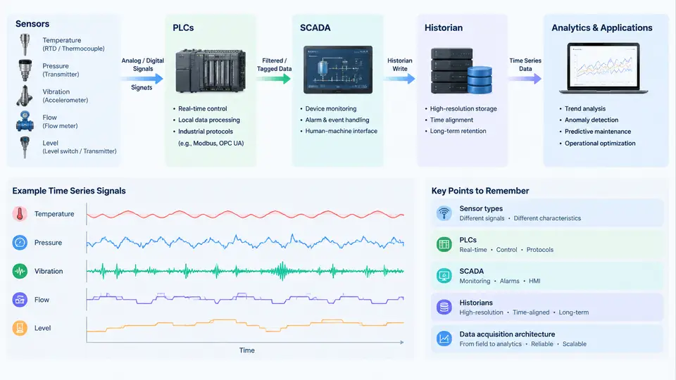
Before any model is trained, any anomaly is detected, or any remaining-useful-life estimate is produced, the data has to come from somewhere. Industrial time series analytics is unusual among machine-learning disciplines because the hardest part is rarely the algorithm — it is understanding the layered, heterogeneous, and often politically fragmented data landscape that sits between a physical machine and an analytics notebook. This chapter maps that landscape: the sensors that generate signals, the controllers that read them, the systems that aggregate them, and the architectures that move them into an analytics environment.
From Physical Phenomenon to Electrical Signal
Every industrial time series begins as a physical quantity. The most common measurement families on rotating and process equipment are:
- Vibration — piezoelectric accelerometers mounted on bearing housings, gearboxes, or motor frames, typically sampled at 10–50 kHz for diagnostics and 1–10 kHz for condition monitoring. Units are m/s² or g.
- Temperature — RTDs (Pt100/Pt1000) and thermocouples on bearings, windings, and lubricant sumps, sampled at 1 Hz or slower.
- Pressure and flow — 4–20 mA transmitters on pumps, compressors, and hydraulic circuits, sampled at 1–100 Hz.
- Speed and position — incremental encoders and proximity probes, often used as the phase reference for order tracking.
- Electrical — current and voltage from motor control centers, sampled at 1–10 kHz for motor current signature analysis.
- Discrete/state — run/stop, valve open/closed, alarm bits, and interlock states, which are essential context for interpreting continuous signals.
The critical engineering point is that these families differ by three to four orders of magnitude in sampling rate and by similar factors in data volume. A single triaxial accelerometer at 25.6 kHz produces roughly 150,000 samples per second; a temperature transmitter produces one. Any acquisition architecture must handle both without forcing the slow signal into the fast pipeline or vice versa.
PLCs, SCADA, and Historians: Three Distinct Roles
These three terms are often used interchangeably in conversation, but they occupy different layers and impose different constraints on analytics.
A Programmable Logic Controller (PLC) executes deterministic control logic in a scan cycle, typically 1–50 ms. It reads I/O, computes, and writes outputs. The PLC is the authoritative source of truth for machine state, but it is not a data store: it holds current values in registers, and only a small subset is exposed to external systems. When you request data from a PLC, you are reading a snapshot of tags, not a history.
SCADA (Supervisory Control and Data Acquisition) is the supervisory layer: HMI displays, alarm management, operator setpoints, and often the OPC server that brokers communication between PLCs and higher-level systems. SCADA is optimized for human latency — one-second updates are typical, and sub-second data is usually discarded.
A historian is a purpose-built time series database designed for industrial data. It stores compressed, timestamped tag values with high write throughput and long retention. Classic historians (OSIsoft PI, Honeywell PHD, Wonderware InSQL) use proprietary compression such as swinging-door or deadband algorithms. Modern alternatives include open-source options like TimescaleDB, InfluxDB, and Apache IoTDB, which trade some industrial-specific compression for SQL familiarity and cloud-native scaling.
Data Acquisition Architectures
There is no single correct architecture. The choice depends on signal bandwidth, network topology, latency requirements, and whether analytics runs on-premises or in the cloud. Four patterns dominate industrial practice.
1. PLC-centric acquisition. Sensors wire into PLC analog input modules. The PLC scales raw counts to engineering units and exposes tags via OPC UA or Modbus TCP. Suitable for slow signals (temperature, pressure, flow) and for state data. Not suitable for vibration — PLC scan cycles and backplane bandwidth cannot sustain kilohertz sampling.
2. Dedicated DAQ with edge buffering. A separate data acquisition chassis (for example, a National Instruments cDAQ or a vendor-specific vibration card) samples high-rate channels, performs anti-alias filtering, and streams to an edge computer. The edge node buffers locally, computes features (RMS, kurtosis, FFT bands), and forwards either raw windows or features upstream. This is the standard pattern for condition monitoring.
3. Historian-mediated. All data converges into the historian, and analytics reads from it via SQL-like interfaces or REST APIs. Simple and well-governed, but historians are usually configured with compression and deadbands that destroy high-frequency content. Use this path for slow signals and for joining context (state, setpoints) to fast data.
4. Publish-subscribe streaming. OPC UA PubSub, MQTT Sparkplug B, or Kafka-based pipelines move data as events. This decouples producers from consumers and supports both edge and cloud analytics. It requires careful timestamping discipline and schema governance, but scales best across many sites.
Practical Implications for Analytics
Three consequences follow directly from this landscape, and they shape every subsequent chapter.
Timestamp integrity is non-negotiable. A vibration window and a temperature reading must be aligned to a common time base. In practice this means UTC timestamps, NTP or PTP clock discipline at the edge, and explicit documentation of whether a timestamp marks the start, center, or end of a sample window. A one-second offset between a fault event and a state change can invert the label of a training example.
Compression changes the signal. Historians apply deadband compression to reduce storage. A swinging-door compression with a 0.5% deadband on a pressure signal will preserve trends but destroy transient spikes that may be the fault signature. Before using historian data for anomaly detection, inspect the raw archive or the compression configuration. If the compression is unknown, treat the data as trend-only.
Context is a separate data stream. A vibration RMS value of 4.2 mm/s means nothing without knowing whether the machine was running, at what load, and at what speed. State bits, setpoints, and production counts must be acquired and joined. In most real projects, the state data comes from the PLC or SCADA via OPC UA, while the vibration data comes from a separate DAQ path — and the join is done in the analytics layer, not at the source.
Common Failure Modes in Acquisition
When analytics produces poor results, the cause is frequently upstream. Typical symptoms and their acquisition-layer causes include:
| Symptom | Likely Acquisition Cause | Diagnostic Check |
|---|---|---|
| Frequency peaks appear at wrong orders | Incorrect sample rate or speed reference | Verify DAQ sample rate against tachometer pulse count |
| Intermittent gaps in vibration data | Edge buffer overflow or network drop | Check edge disk write latency and broker queue depth |
| Temperature signal looks flat | Historian deadband too wide | Compare raw PLC register against historian trend |
| Labels misaligned with faults | Clock skew between PLC and DAQ | Compare NTP offset logs on both devices |
| Aliased high-frequency content | Missing or inadequate anti-alias filter | Inspect DAQ filter configuration and Nyquist margin |
The acquisition layer is where data quality is won or lost. A model trained on misaligned, over-compressed, or aliased data will fail in ways that are difficult to diagnose from the analytics side alone. The remaining chapters build on this foundation: signal processing assumes clean, correctly sampled waveforms; feature engineering assumes aligned context; and prognostics assumes that the historical record reflects the true operating history of the machine.