1. Industrial sensor data fusion landscape

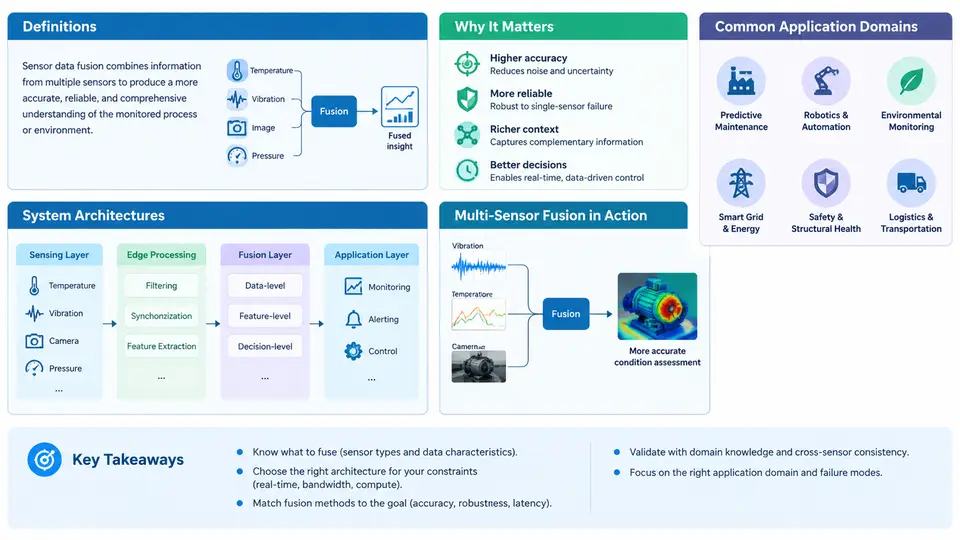
Modern industrial plants rarely rely on a single measurement to make a decision. A gas turbine is monitored by dozens of thermocouples, pressure transmitters, vibration accelerometers, and flow meters; a robotic assembly cell combines encoder counts, force-torque signals, and vision data. Sensor data fusion is the discipline of combining observations from multiple, often heterogeneous, sensors to produce an estimate, classification, or decision that is more accurate, more complete, and more reliable than what any single sensor could deliver alone.

It is important to distinguish fusion from mere data aggregation. Aggregation concatenates readings; fusion exploits redundancy and complementarity. Redundant sensors observe the same physical quantity and allow noise averaging and fault detection. Complementary sensors observe different quantities that jointly describe a state — for example, temperature plus vibration to characterize bearing health. Cooperative sensors, such as a stereo camera pair, must be combined to yield information (depth) that neither provides independently.

Why Fusion Is Necessary in Industrial Settings

Four motivations dominate real deployments. First, accuracy and uncertainty reduction: averaging N independent measurements with variance σ² reduces the fused variance toward σ²/N under ideal conditions. Second, coverage and observability: no single modality sees everything, so fusion extends the measurable state space. Third, robustness and fault tolerance: when one sensor drifts or fails, cross-checking against others preserves operation. Fourth, latency and cost trade-offs: fusing a cheap fast sensor with a slow accurate one can meet both timing and precision budgets.

System Architectures

Fusion architectures are commonly classified by where fusion occurs in the signal chain. In centralized fusion, raw measurements from all sensors are transmitted to one node that performs alignment and estimation. This yields optimal estimates but demands high bandwidth and tight time synchronization. In decentralized (distributed) fusion, each sensor or local node computes a partial estimate (e.g., a local Kalman filter) and only these estimates are shared, drastically reducing communication at the cost of some optimality. Hierarchical fusion layers the two: local nodes fuse their own clusters, and a higher-level node fuses the cluster outputs — the dominant pattern in plant-wide systems.

A second axis is the level of fusion. Data-level (low-level) fusion combines raw signals before any interpretation. Feature-level (intermediate) fusion combines extracted features such as RMS vibration, spectral peaks, or edge descriptors. Decision-level (high-level) fusion combines the outputs of independent classifiers or detectors, for instance via voting or Bayesian combination. The choice depends on sensor homogeneity, bandwidth, and how much preprocessing is feasible at the edge.

Timing is the hidden engineering constraint. Fused data must refer to the same instant, so architectures include timestamping, buffering, and interpolation. A common approach is to timestamp every sample at the source using a synchronized clock (e.g., IEEE 1588 PTP) and resample onto a common grid before fusion.

Application Domains

Fusion appears across the industrial lifecycle. In condition monitoring and predictive maintenance, vibration, temperature, and acoustic emission are fused to estimate remaining useful life of bearings and gearboxes. In process control, redundant and complementary measurements feed soft sensors and model predictive controllers. In robotics and automation, IMU, encoder, force-torque, and vision data are fused for state estimation and safe manipulation. In quality inspection, 2D/3D vision plus spectral sensing detects surface and subsurface defects. In energy and utilities, phasor measurement units and SCADA telemetry are fused for grid state estimation. In safety and environmental monitoring, gas, flame, and thermal sensors are fused to reduce false alarms.

A Concrete Fusion Example

Consider estimating the temperature of a bearing housing using two sensors: a fast thermocouple with noise σ₁ = 1.5 °C and a slower RTD with σ₂ = 0.8 °C. Under a simple inverse-variance weighting, the fused estimate is:

w1 = (1/σ1²) / (1/σ1² + 1/σ2²) = (1/2.25) / (1/2.25 + 1/0.64) ≈ 0.221
w2 = 1 - w1 ≈ 0.779
T_fused = w1 * T1 + w2 * T2

If T1 = 72.0 °C and T2 = 70.5 °C, then T_fused ≈ 0.221×72.0 + 0.779×70.5 ≈ 70.83 °C, with a fused variance of about 0.49 °C² (σ ≈ 0.70 °C) — better than either sensor alone. In practice, you would also check the innovation (residual) between each sensor and the fused value; a persistent residual beyond three sigma signals drift or a fault, triggering recalibration or sensor replacement.

Key Takeaways

• Fusion combines redundant, complementary, and cooperative sensors to improve accuracy, coverage, and robustness.
• Architectures differ by location (centralized, decentralized, hierarchical) and by level (data, feature, decision).
• Time synchronization, calibration, and outlier handling are prerequisites, not optional steps.
• Industrial applications span condition monitoring, process control, robotics, inspection, energy, and safety.
• Always report a fused estimate together with its uncertainty and validate against residuals.