1. Industrial KPI analytics and dashboard e
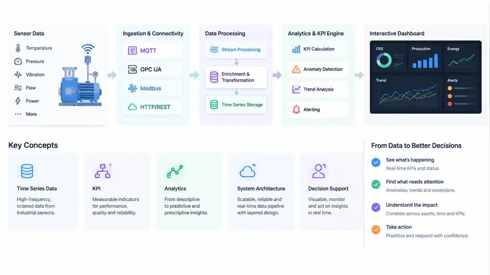
Industrial KPI analytics is the discipline of turning raw measurements collected from production assets into a small set of trustworthy, continuously updated performance indicators that operators, engineers, and plant managers can act on. Dashboard engineering is the complementary practice of designing, building, and operating the software layer that computes those indicators and presents them as interactive decision support. The two are inseparable: a well-designed dashboard fed by unreliable KPI logic is worse than no dashboard at all, because it creates false confidence. This chapter establishes the vocabulary, the reference architecture, and the end-to-end workflow that the remaining chapters will implement in detail.
What Counts as an Industrial KPI
Not every measurement is a KPI. A KPI is a derived, time-bounded quantity that expresses how well an asset, line, or plant is performing against a defined target. Typical examples in discrete and process manufacturing include Overall Equipment Effectiveness (OEE), scrap rate, first-pass yield, mean time between failures (MTBF), specific energy consumption per unit produced, and schedule adherence. Each of these shares four properties:
- Derived: it is computed from one or more raw signals plus contextual data such as production counts, shift calendars, or product recipes.
- Time-bounded: it is always evaluated over an explicit interval — a shift, an hour, a batch, or a rolling window.
- Comparable: it has a target, a baseline, or a historical distribution against which the current value can be judged.
- Actionable: a deviation points to a specific investigation or intervention.
Raw tags such as Motor_Temp_C or Line_Speed_mps are inputs, not KPIs. The transformation from tag to KPI is where most engineering effort and most errors live.
Reference System Architecture
A production-grade industrial KPI platform is usually organized into five layers. Understanding the responsibility of each layer prevents the common mistake of pushing business logic into the wrong place.
| Layer | Responsibility | Typical Technology |
|---|---|---|
| Edge / acquisition | Read PLC and sensor tags, timestamp at source, buffer during network loss | OPC UA server, Modbus gateway, edge agent |
| Transport & storage | Move and persist time-series and contextual data | MQTT/Sparkplug B, historian, time-series database |
| KPI computation | Apply state models, counters, and aggregation logic | Stream processor, SQL/continuous query engine |
| Semantic / context | Map tags to assets, shifts, products, and units | Asset model, tag registry, unit metadata |
| Presentation | Serve interactive views, alerts, and drill-down | Web dashboard, API layer, alerting service |
The critical design rule is that KPI logic belongs in the computation layer, not in the dashboard. If OEE is calculated inside a chart widget, every new view re-implements the formula and the numbers will eventually disagree. Compute once, serve many.
The End-to-End Workflow: From Sensor to Decision
The workflow below is the backbone of this course. Each stage has a distinct failure mode, and the SVG illustrates how data and context flow through them.
- Acquisition. A sensor or PLC exposes a value with a source timestamp. Sampling may be cyclic (every 100 ms) or on-change. The edge agent must preserve the source timestamp, not the arrival time, because network jitter would otherwise distort duration-based KPIs.
- Contextualization. The raw tag is bound to an asset (Line 3 Filler), a unit (bar), and a production context (shift B, product SKU-4471). Without this binding, a count of 12,000 bottles cannot be interpreted.
- State classification. Many KPIs depend on whether the asset is Running, Idle, Down, or Blocked. This is derived from a combination of signals — for example, speed > 0.5 m/s and no fault word set means Running. State logic is the most common source of KPI disputes.
- KPI computation. Counters and durations are aggregated over the evaluation window. OEE, for instance, is Availability × Performance × Quality, each of which is itself a ratio of accumulated times or counts.
- Storage and versioning. Computed KPI values are written back to the time-series store with the formula version attached, so historical values remain reproducible after a formula change.
- Presentation and interaction. The dashboard queries the KPI store, renders trends and gauges, and supports drill-down from plant to line to asset to raw tag.
- Decision and feedback. An operator acts — adjusts a setpoint, calls maintenance, changes a schedule — and the effect appears in the next evaluation window, closing the loop.
Worked example (illustrative values). Consider a filling line evaluated over a one-hour window. The line was scheduled for 60 minutes. State logic records 48 minutes Running, 8 minutes Idle (no product), and 4 minutes Down (filler fault). The ideal rate is 200 bottles/min; actual good bottles counted = 9,120, total bottles produced = 9,600.
- Availability = 48 / 60 = 0.800
- Performance = 9,600 / (48 × 200) = 9,600 / 9,600 = 1.000
- Quality = 9,120 / 9,600 = 0.950
- OEE = 0.800 × 1.000 × 0.950 = 0.760
The dashboard would show OEE 76.0%, with Availability as the dominant loss. Drilling into the 4-minute Down interval should reveal the filler fault code and the 8-minute Idle interval should be checked against the production schedule — if no product was planned, that time should arguably be excluded from scheduled time, which would raise Availability. This is exactly the kind of semantic decision that must be made explicitly and documented.
Key Concepts and Vocabulary
Several terms recur throughout the course and are worth fixing now. Tag refers to a single named signal. Asset model is the hierarchy of enterprise, site, area, line, and equipment. Evaluation window is the time interval over which a KPI is computed. Counter is a monotonically increasing value (total bottles) that must be differenced, with rollover handling. State model is the finite set of equipment states and the rules that assign them. Drill-down path is the navigation route from aggregate KPI to contributing raw data. Data latency is the delay between physical event and dashboard update, and it directly limits how quickly a decision can be made.
Common pitfall. Mixing source timestamps and arrival timestamps in the same aggregation. If the edge buffer replays 30 seconds of data after a network outage, arrival-time aggregation will compress those 30 seconds into one, inflating rates. Always aggregate on source time and record the replay event.
What the Dashboard Must Deliver
An interactive industrial dashboard is not a reporting page. It must answer three questions within seconds: Are we on target right now? If not, where is the loss? What changed recently? This implies a layered view — a plant overview with status colors, a line view with KPI trends and loss breakdown, and an asset view with raw signals and state timeline. Interactivity means filtering by shift, product, and time range, and drilling from any aggregate to its contributors. The engineering challenge is keeping all layers consistent: the same OEE value must appear whether it is read from the overview tile or recomputed from the asset view.
Engineering Implications
Three implications follow from this architecture. First, timestamp discipline is non-negotiable; every downstream KPI inherits the quality of the time base. Second, state logic must be explicit and testable — it should be expressed as rules with named inputs, not buried in conditional code. Third, the semantic layer is a first-class asset; when a line is re-tagged or a product is re-routed, the asset model must be updated in the same change window as the physical modification, or KPIs will silently attribute production to the wrong asset.
With this foundation — KPI definition, layered architecture, and the seven-stage workflow — the following chapters will move into acquisition details, state modeling, formula implementation, storage design, and interactive dashboard construction, each building on the same reference model.