1. Engineering data profiling fundamentals
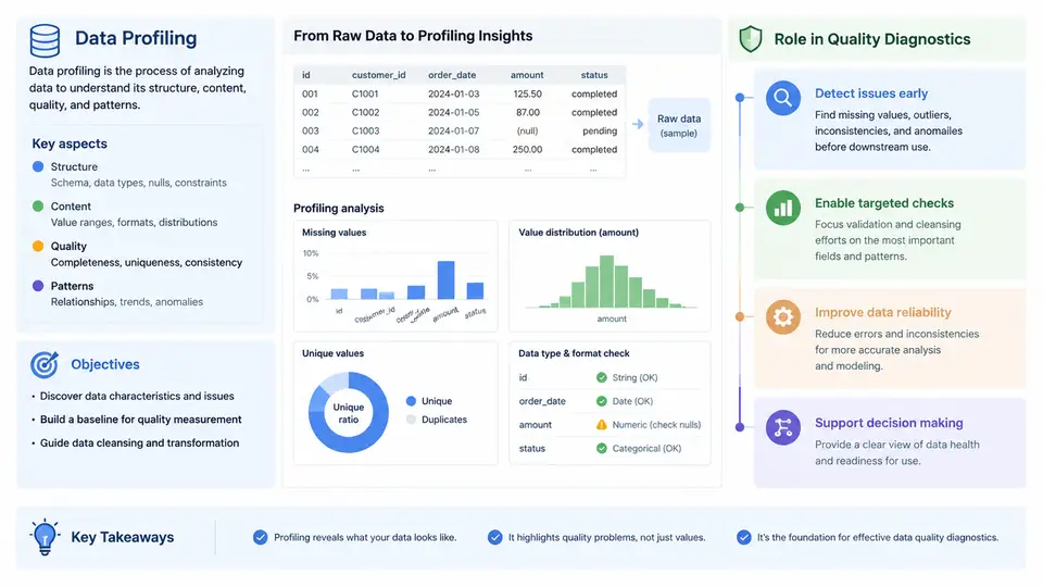
Data profiling is the systematic process of examining a dataset to collect statistical summaries, structural metadata, and content-level characteristics that describe what the data actually contains. In an engineering context, profiling is not a one-time exploratory step performed by an analyst out of curiosity; it is a repeatable, instrumented procedure that produces measurable evidence about data condition. The output of profiling — column statistics, value distributions, pattern frequencies, key candidates, and cross-column dependencies — becomes the factual baseline against which data quality diagnostics are performed.
It is useful to separate three related activities that are often conflated:
- Profiling answers “what is in this dataset?” It is descriptive and largely non-judgmental. A column may be 12% null; profiling reports that fact without declaring it a defect.
- Quality diagnostics answers “does this dataset meet its declared or implied requirements?” It compares profiled facts against rules, contracts, or expectations and classifies deviations.
- Monitoring answers “has the condition changed since the last accepted baseline?” It applies profiling statistics over time and detects drift.
Profiling therefore supplies the evidence; diagnostics supply the verdict. Without a profiling baseline, a diagnostic rule such as “null rate must be below 2%” has no grounding, and a drift alert has no reference point.
Objectives of Engineering Data Profiling
In production data engineering, profiling serves several concrete objectives. Each maps to a class of metadata that downstream systems consume.
| Objective | Profiled artifact | Typical downstream use |
|---|---|---|
| Establish structural inventory | Column count, data types, ordinal position, nullability | Schema comparison, migration validation |
| Quantify completeness | Null count and null rate per column, empty-string rate | Completeness SLAs, imputation planning |
| Characterize value domains | Distinct count, cardinality ratio, top-K values, min/max | Enumeration checks, categorical encoding |
| Detect format and pattern structure | Regex pattern frequency, length distribution | Format validation rules, parsing logic |
| Identify candidate keys | Uniqueness ratio, composite uniqueness | Primary key selection, deduplication |
| Reveal dependencies | Functional dependency candidates, correlation | Normalization, join-path discovery |
A practical profiling run on a table such as orders might produce, for the column customer_id: 1,000,000 rows, 0 nulls, 998,412 distinct values, uniqueness ratio 0.9984, minimum length 8, maximum length 8, and a single dominant pattern ^C[0-9]{7}$ covering 99.97% of values. That single profile immediately raises a diagnostic question: why are there 1,588 duplicate customer_id values in an order table? Profiling did not answer the question, but it made the question precise and testable.
Where Profiling Sits in the Quality Diagnostic Workflow
Profiling is the first stage of a four-stage diagnostic loop. The stages are not merely sequential; findings from later stages frequently send the engineer back to refine the profile.
What a Profiling Pass Actually Computes
Profiling is not a single query. It is a set of column-level and table-level aggregations. For a relational source, a minimal engineering profile computes the following per column:
-- Column-level profile (PostgreSQL syntax, illustrative)
SELECT
  COUNT(*)                                   AS row_count,
  COUNT(*) - COUNT(customer_id)              AS null_count,
  ROUND(100.0 * (COUNT(*) - COUNT(customer_id)) / COUNT(*), 3)
                                             AS null_pct,
  COUNT(DISTINCT customer_id)                AS distinct_count,
  ROUND(COUNT(DISTINCT customer_id)::numeric
        / NULLIF(COUNT(customer_id), 0), 4)  AS uniqueness_ratio,
  MIN(LENGTH(customer_id))                   AS min_len,
  MAX(LENGTH(customer_id))                   AS max_len
FROM orders;
Running this against a sample orders table with 1,000,000 rows might return row_count = 1000000, null_count = 0, null_pct = 0.000, distinct_count = 998412, uniqueness_ratio = 0.9984, min_len = 8, max_len = 8. These are illustrative values, not measured results, but they demonstrate the shape of the output. The uniqueness_ratio of 0.9984 is the trigger for a diagnostic rule: if customer_id is expected to be unique per order, the rule uniqueness_ratio ≥ 0.9999 fails, and the 1,588 duplicate values become the investigation target.
Pattern profiling extends this by sampling values and grouping them by regular-expression shape. A frequency table of patterns for customer_id might show:
| Pattern | Match count | Share |
|---|---|---|
^C[0-9]{7}$ |
999,700 | 99.97% |
^c[0-9]{7}$ |
180 | 0.018% |
^C[0-9]{6}$ |
120 | 0.012% |
The lowercase c prefix and the six-digit suffix are both format deviations. Profiling surfaced them without any prior rule; the diagnostic stage then decides whether they are defects (they almost certainly are, given the dominant pattern) and what remediation applies.
Profiling as the Foundation of Diagnostics
The relationship between profiling and diagnostics can be stated precisely: profiling produces measurements; diagnostics evaluates measurements against requirements. A diagnostic rule is only as good as the profile that feeds it. If the profile does not compute uniqueness_ratio, no uniqueness rule can fire. If the profile samples only the first 10,000 rows, a rare but critical pattern in the tail will be missed.
Deliverable: Column Profiling Record
The following record is a reusable artifact for capturing a single column profile in a form that diagnostics can consume directly. It is intentionally minimal and contains only fields relevant to engineering data quality work.
| Field | Example value | Diagnostic role |
|---|---|---|
source_table |
orders |
Locates the profiled object |
column_name |
customer_id |
Identifies the profiled attribute |
row_count |
1000000 | Denominator for all rates |
null_pct |
0.000 | Completeness rule input |
uniqueness_ratio |
0.9984 | Key-candidate rule input |
dominant_pattern |
^C[0-9]{7}$ |
Format rule input |
pattern_coverage |
0.9997 | Threshold for format conformance |
profiled_at |
2025-01-15T09:30:00Z | Drift baseline timestamp |
With this record in place, a diagnostic rule is a simple comparison: uniqueness_ratio < 0.9999 → FAIL, pattern_coverage < 0.999 → WARN, null_pct > 0.02 → FAIL. The profile supplies the left-hand side; the contract supplies the right-hand side. That separation is what makes engineering data profiling a repeatable discipline rather than an ad-hoc inspection.
The next chapter builds on this foundation by examining the specific statistical measures — cardinality, distribution shape, and dependency metrics — that a production profiling engine computes, and how each measure maps to a class of data quality defect.