1. Foundations of causal inference in indus

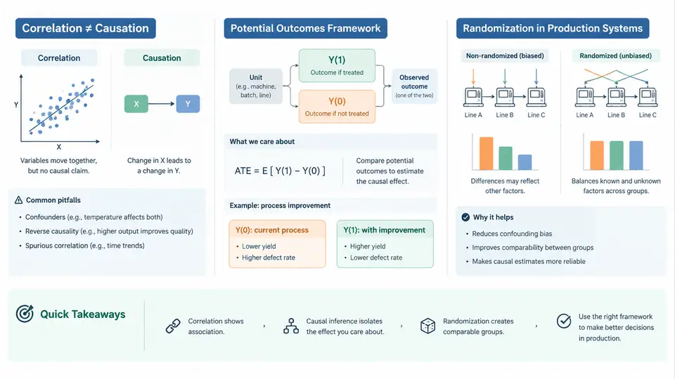
Every process engineer has encountered a version of the same trap: a parameter is adjusted, yield improves, and the adjustment is credited with the gain. Weeks later, the improvement evaporates. The parameter was never the cause. Something else moved at the same time — a raw material lot change, a seasonal ambient humidity shift, a recalibrated sensor — and the process responded to that instead. Distinguishing correlation from causation is not an academic exercise in a factory; it is the difference between a fix that holds and a fix that fails on the next production run.

Why Correlation Is Not Enough on the Shop Floor

Consider an injection molding line tracking cavity pressure and part weight. Historical data show a strong positive correlation (r ≈ 0.87) between peak cavity pressure and part weight. It is tempting to conclude that raising pressure increases weight, and to "tune" the process by pushing pressure up. But both variables are driven by a common cause: melt viscosity, which itself depends on barrel temperature and resin moisture content. Pressure and weight move together because viscosity moves them together. Adjusting pressure alone changes the pressure reading without reliably changing the underlying physics that determines fill quality.

This structure — a confounder influencing both the presumed cause and the effect — is the single most common reason process correlations mislead. Three other patterns recur just as often:

• Reverse causation: Operators increase cooling time when they observe warpage. The data then show cooling time correlated with warpage, but the causality runs backward — warpage is causing the adjustment, not the reverse.
• Selection effects: Only parts that pass a preliminary inspection reach final dimensional measurement. Correlations computed on this filtered dataset describe the inspection gate, not the process.
• Coincident drift: Two variables both trend with tool wear or ambient temperature over a shift, producing correlation with no direct link.

The practical consequence is that a regression coefficient, a correlation matrix, or a control chart pattern is evidence of association, never proof of mechanism. Causal claims require an explicit framework that states what would happen under intervention.

The Potential Outcomes Framework

The potential outcomes framework gives that rigor a precise language. For each unit — a part, a batch, a wafer, a production run — define two potential outcomes:

• Y(1): the outcome if the unit receives the treatment (e.g., new parameter setpoint, new supplier lot, revised cure profile).
• Y(0): the outcome if the unit receives the control condition.

The individual causal effect is Y(1) − Y(0). The fundamental problem is that we can never observe both for the same unit: once a batch is run at the new setpoint, its counterfactual outcome under the old setpoint is gone. This is the fundamental problem of causal inference, and it is not a data-quality issue — it is structural.

Because individual effects are unobservable, we estimate average treatment effects across comparable groups. The estimand for a population is:

ATE = E[Y(1) − Y(0)]
    = E[Y(1)] − E[Y(0)]

This quantity is only recoverable if the treated and control groups are exchangeable — if, before treatment, they would have had the same average outcome. Formally, we need independence: treatment assignment must be independent of potential outcomes, written as (Y(1), Y(0)) ⟂ T. When that holds, the naive difference in observed means equals the causal effect. When it fails, the difference is contaminated by confounding, and no amount of additional data from the same observational design will remove the bias.

Randomization as the Engine of Identification

Randomization is the most reliable way to establish exchangeability. If treatment assignment is genuinely random, then confounders — measured and unmeasured alike — are balanced in expectation across groups. This is why randomized controlled trials are the reference standard, and why designed experiments (DOE) occupy the same role in manufacturing.

In a production setting, randomization does not mean chaos. It means that the assignment of units to conditions is determined by a mechanism independent of the outcome. A practical example: a 2² factorial screening experiment on a soldering process, with two factors — peak reflow temperature (A) and conveyor speed (B) — each at two levels. Sixteen boards are run, and the run order is randomized rather than grouped by factor level.

Run order (randomized):  A    B    Yield (%)
1                        210  80   94.2
2                        230  80   96.1
3                        210  100  93.8
4                        230  100  97.4
5                        230  80   95.8
6                        210  100  94.0
7                        230  100  97.1
8                        210  80   94.5
... (8 additional runs, randomized)

Randomizing run order protects against nuisance variables that drift over time — operator fatigue, paste aging, ambient humidity. If all high-temperature runs were performed first, a temperature effect would be indistinguishable from a time effect. Randomization breaks that aliasing.

Three practical constraints shape how randomization is applied in manufacturing:

1. Hard-to-change factors. Furnace temperature, for instance, may take hours to stabilize. Fully randomizing every run is impractical. Split-plot designs randomize hard-to-change factors at the whole-plot level and easy-to-change factors within plots, accepting a known variance structure in exchange for feasibility.
2. Ethical and safety limits. You cannot randomize operators to an unsafe condition or randomize patients to a defective implant. Here, observational methods with explicit assumptions — propensity scores, instrumental variables, difference-in-differences — become necessary.
3. Throughput cost. Every experimental run displaces salable production. Randomization must be justified by the value of the information it produces, which is why screening designs use the minimum runs needed to estimate main effects.

From Association to Intervention: A Decision Path

The figure below maps the reasoning path from an observed correlation to a defensible causal claim, showing where randomization and its alternatives enter.

What This Means for Process Improvement Work

The framework changes how you read data and how you plan experiments. Three habits follow directly:

• State the intervention before analyzing. Write down the treatment, the outcome, and the comparison condition. If you cannot articulate what "doing X instead of Y" means physically, you do not yet have a causal question.
• Ask what could confound the comparison. List plausible common causes of both the factor and the response. If any are uncontrolled, either randomize or measure and adjust for them — and be honest about what remains unmeasured.
• Prefer design over adjustment when feasible. Randomization and blocking are cheaper and more credible than post-hoc statistical correction. Reserve observational methods for constraints that genuinely prevent experimentation.

The remainder of this course builds on these foundations. Later chapters develop identification strategies for observational process data, design and analysis of industrial experiments, and methods for validating causal claims against production reality. The vocabulary introduced here — potential outcomes, exchangeability, confounding, and the primacy of randomization — will recur throughout, because every credible process improvement rests on them.