1. Simulation and test data landscape
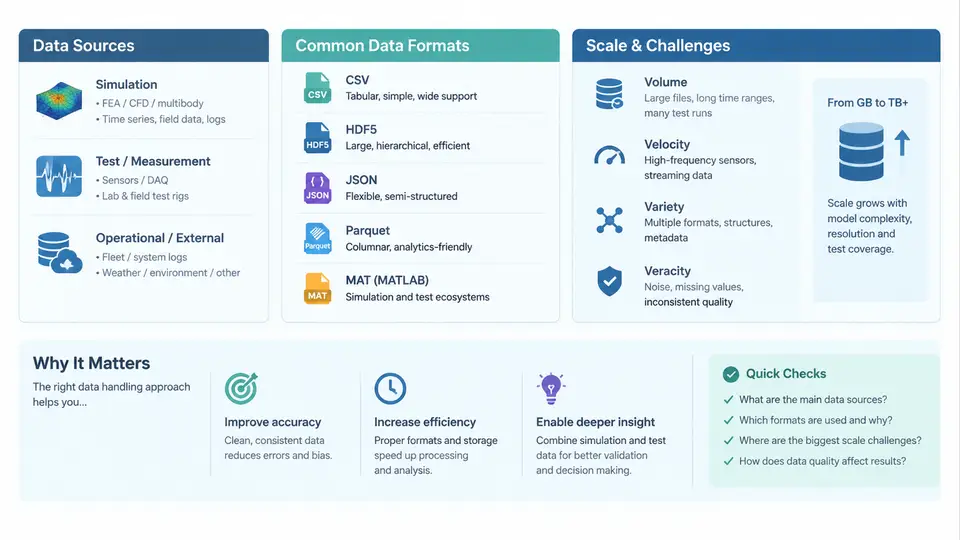
Engineering organizations that run simulations and physical tests generate data at a rate that consistently outpaces the infrastructure built to store and analyze it. A single transient structural analysis may emit hundreds of gigabytes of time-series output; a wind-tunnel campaign with hundreds of pressure taps and accelerometers can produce terabytes over a few weeks. Before any processing pipeline can be designed, it is necessary to understand where this data originates, what forms it takes, and why conventional data-handling approaches break down at scale. This chapter maps that landscape and establishes the vocabulary used throughout the course.
Primary Data Sources in Engineering Workflows
Simulation and test data comes from several distinct source families, each with its own generation cadence, fidelity characteristics, and metadata conventions.
- Numerical simulation (CAE): Finite element analysis (FEA), computational fluid dynamics (CFD), multibody dynamics, and electromagnetic solvers. Outputs include nodal/element fields, time histories, modal results, and solver logs. Typical tools: Ansys, Abaqus, Nastran, OpenFOAM, LS-DYNA.
- Physical test and measurement: Strain gauges, accelerometers, thermocouples, pressure transducers, and digital image correlation systems. Data arrives as high-rate time series, often through DAQ systems such as National Instruments PXI or HBM catman.
- Sensor and telemetry streams: Vehicle, aircraft, or rig telemetry with CAN bus, ARINC 429, or Ethernet-based protocols, producing continuous multi-channel records.
- Hybrid and co-simulation: Hardware-in-the-loop (HIL) and software-in-the-loop setups that couple physical hardware with simulated environments, generating interleaved real-time and simulated signals.
- Derived and post-processed data: Reduced-order models, surrogate training sets, fatigue cycle counts, and statistical summaries produced downstream.
Each source carries different metadata obligations. A CFD run needs mesh topology, solver version, turbulence model, and boundary conditions recorded alongside the field data. A strain-gauge test needs channel calibration factors, sampling rates, and physical units. Losing this context renders the raw numbers nearly useless for later correlation or regression testing.
Data Formats: A Fragmented Ecosystem
There is no universal format in this domain. The format landscape reflects decades of tool-specific evolution, and interoperability remains a persistent engineering challenge.
| Category | Common Formats | Characteristics |
|---|---|---|
| FEA results | ODB, .rst, .op2, .h5 | Binary, solver-specific, large per-timestep |
| CFD results | CGNS, EnSight, VTK, OpenFOAM | Mesh + field, often parallel-partitioned |
| Test time series | MDF4, TDMS, HDF5, CSV | Channel-oriented, high sample rates |
| Telemetry | CAN log (BLF, ASC), Parquet | Bus-oriented, event-timestamped |
| Interchange | STEP, IGES, STL | Geometry only, no results |
The practical consequence is that a correlation study comparing simulated strain against measured strain may require reading ODB, MDF4, and CSV files in the same pipeline, then reconciling time bases, units, and coordinate systems. Format fragmentation is not a minor inconvenience; it is a primary driver of pipeline complexity.
Scale Challenges
Three dimensions of scale stress engineering data infrastructure simultaneously.
Volume. A single CFD transient with 50 million cells and 10,000 timesteps, storing 5 fields per cell in double precision, yields roughly 50M × 10,000 × 5 × 8 bytes ≈ 20 TB before compression. Multiply by parametric sweeps and design-of-experiments campaigns, and storage requirements reach petabytes.
Velocity. HIL rigs and telemetry streams produce data continuously during a test. If a rig has 200 channels sampled at 50 kHz, that is 10 million samples per second, or about 80 MB/s in 64-bit floats. Sustained ingestion at this rate requires streaming architectures rather than batch file writes.
Variety. The same physical event may be represented as a structured time series, an unstructured mesh field, a set of scalar KPIs, and a text log. Joining these representations for a single analysis requires schema reconciliation across fundamentally different data models.
From Raw Files to Queryable Data
The central architectural insight of this course is that raw simulation and test files should be treated as landing data, not as the analytical substrate. The practical pattern is to ingest raw files, extract structured records (channels, timesteps, scalar fields, metadata), and write them into columnar or array-oriented stores that support efficient slicing and aggregation.
Consider a concrete example. A test campaign produces 400 MDF4 files, each containing 120 channels at 10 kHz for 30 seconds. Naive processing reads each file fully into memory, which is wasteful when the analyst only needs channels 7, 12, and 45 for a specific time window. A better approach parses the MDF4 metadata first, builds an index of channel-to-file-and-offset mappings, and then reads only the required byte ranges. In HDF5 or Parquet, this becomes a predicate pushdown and column projection problem, and query time drops by one to two orders of magnitude.
# Illustrative ingestion sketch (pseudo-code)
for mdf_file in campaign.glob("*.mf4"):
    meta = read_mdf4_metadata(mdf_file)          # channels, units, rate
    index.append({
        "file": mdf_file.name,
        "channels": meta.channel_names,
        "rate_hz": meta.sample_rate,
        "start_time": meta.trigger_time,
        "bytes": mdf_file.stat().st_size,
    })
write_index(index, "campaign_index.parquet")

# Later: read only needed channels and window
subset = read_mdf4_channels(
    "run_017.mf4",
    channels=["strain_07", "accel_12", "press_45"],
    t_start=4.2, t_end=4.8,
)
The index itself is small and fast to query; the heavy data stays in its original files until a specific analytical need justifies reading it. This separation of catalog from payload is foundational.
Metadata and Provenance as First-Class Concerns
At scale, data without metadata is indistinguishable from noise. Every record in a well-designed pipeline should be traceable to its source file, solver or DAQ version, calibration state, and processing history. This is not bureaucratic overhead; it is what makes correlation, regression, and reproducibility possible. When a test engineer asks "why does the simulated peak stress differ from the measured peak by 18%?", the answer depends on being able to retrieve the exact boundary conditions, material model, and sensor calibration used in each case.
Visualizing the Data Flow
The diagram below summarizes how data moves from source systems through ingestion into analytical stores, and where the principal scale pressures act.
What This Means for Processing Design
Three design principles follow directly from the landscape described above. First, decouple catalog from payload: maintain a lightweight, queryable index of what data exists and where, separate from the heavy raw files. Second, normalize at ingestion, not at query time: convert units, align time bases, and record provenance once, so downstream consumers do not each re-solve the same reconciliation problems. Third, choose storage formats that match access patterns: columnar formats for channel-oriented time series, array stores for mesh fields, and relational or catalog databases for metadata and lineage.
These principles recur throughout the course. The chapters that follow apply them to specific stages: ingestion pipelines, distributed processing, correlation workflows, and machine-learning feature extraction. The landscape itself—fragmented formats, heterogeneous sources, and relentless scale growth—is the problem this course exists to solve.