1. Bayesian reliability framework for field
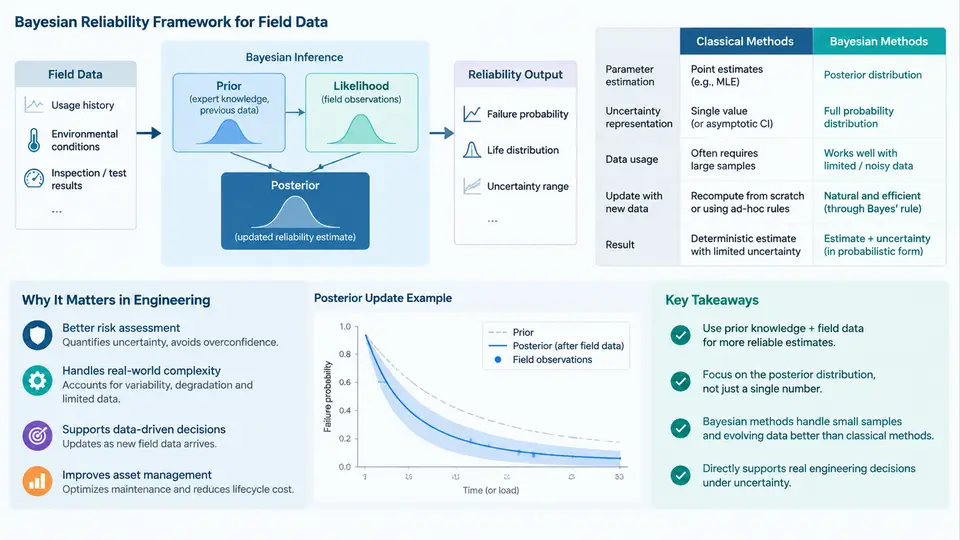
Field reliability data rarely arrive as a clean, balanced experiment. They come from units already deployed, with staggered entry times, incomplete failure records, mixed operating profiles, and maintenance actions that alter the failure process itself. The Bayesian reliability framework treats this messiness as information rather than noise: it combines a prior distribution encoding engineering knowledge with a likelihood function built from the observed field data, producing a posterior distribution over the reliability parameters of interest. That posterior is the complete inferential object — every reliability metric (reliability at time t, hazard rate, mean time to failure, warranty return rate) is derived from it by integration or simulation.
Fundamental Principles
Bayes' theorem for reliability parameters takes the form
p(θ | D) = p(D | θ) · p(θ) / p(D)

θ  : parameter vector (e.g., Weibull shape β and scale η)
D  : observed field data (failure times, censoring times, covariates)
p(θ)   : prior distribution — engineering knowledge before seeing D
p(D|θ) : likelihood — probability of the observed data given θ
p(θ|D) : posterior — updated knowledge after seeing D
p(D)   : normalizing constant, ∫ p(D|θ)p(θ) dθ
Three principles distinguish this from a purely mechanical application of the formula. First, probability is a degree of belief, not only a long-run frequency, so it is legitimate to state "there is a 90% probability that the B10 life exceeds 8,000 hours." Second, all uncertainty is propagated: parameter uncertainty flows into every prediction, so a credible interval on reliability is produced directly rather than bolted on afterward. Third, information is cumulative: yesterday's posterior becomes today's prior, which is exactly how a fleet's reliability knowledge should evolve as field returns accumulate.
How It Differs from Classical Methods
Classical (frequentist) reliability analysis treats θ as a fixed unknown constant and asks what long-run frequency of datasets would produce the observed result. The Bayesian approach treats θ as a random variable with a distribution. The practical consequences are substantial for field data.
| Aspect | Classical (MLE / frequentist) | Bayesian |
|---|---|---|
| Parameter interpretation | Fixed unknown constant | Random variable with a distribution |
| Small-sample behavior | Estimates unstable; intervals may be wide or undefined | Prior stabilizes estimates; intervals remain valid |
| Prior knowledge | Not formally usable | Encoded explicitly and auditable |
| Censoring / truncation | Handled via specialized likelihoods | Same likelihood, naturally combined with prior |
| Interval meaning | Confidence interval: coverage over repeated samples | Credible interval: direct probability statement about θ |
| Prediction | Plug-in estimate, uncertainty often ignored | Posterior predictive distribution includes all uncertainty |
| Sequential updating | Re-analyze from scratch | Posterior → prior, incremental |
The most consequential difference in practice is the treatment of small samples and heavy censoring. A field campaign may yield 12 failures out of 400 shipped units, with the remaining 388 right-censored at various ages. Maximum likelihood can still fit a Weibull model, but the confidence interval on the shape parameter may span an order of magnitude, and the B10 life estimate can be physically implausible. A Bayesian model with a weakly informative prior on β (say, lognormal centered near 1.5 with moderate spread) keeps the estimate in a defensible region while still letting the data dominate when evidence is strong.
Engineering Motivation
Field data are expensive, sparse, and structurally awkward. Three engineering realities make the Bayesian framework the natural choice.
- You already have prior knowledge. Similar products, bench tests, supplier data, and physics-of-failure models all constrain what the field failure rate can plausibly be. Discarding that knowledge is not neutral — it wastes information.
- Decisions must be made now. A warranty reserve, a redesign trigger, or a maintenance interval cannot wait for 10,000 failures. Bayesian inference gives a defensible answer with the data at hand, plus an honest statement of remaining uncertainty.
- Data arrive continuously. Field returns stream in monthly. The posterior from last month is the prior for this month, so the reliability estimate updates smoothly instead of jumping between disjoint analyses.
Worked Example: Weibull Analysis of Field Returns
Consider a fleet of 500 industrial pumps. Over 18 months, 14 units failed; the remaining 486 are right-censored at their current operating hours. Assume a Weibull life model with shape β and scale η (hours), and a weakly informative prior:
β ~ LogNormal(μ = log(1.5), σ = 0.5)
η ~ LogNormal(μ = log(20000), σ = 1.0)

Likelihood for each failed unit i:   f(t_i | β, η)
Likelihood for each censored unit j: S(t_j | β, η) = exp(-(t_j/η)^β)

Posterior: p(β, η | D) ∝ p(β) p(η) ∏ f(t_i) ∏ S(t_j)
With failure times ranging from 3,200 to 15,800 hours and censoring times from 1,000 to 18,000 hours, a Metropolis–Hastings sampler with 20,000 iterations (5,000 burn-in) yields a posterior median near β ≈ 1.7 and η ≈ 24,000 hours. The 90% credible interval on B10 life might be, for example, 6,500–11,200 hours. The exact numbers depend on the data; the point is that the output is a distribution, not a single number, and it directly supports a statement such as "the probability that B10 life is below 8,000 hours is 0.18."
To reproduce this analysis, the essential steps are: (1) assemble failure and censoring times with consistent age definitions; (2) specify priors and justify them; (3) code the likelihood with censoring; (4) sample the posterior; (5) check convergence (trace plots, R-hat); (6) run posterior predictive checks against the observed data; (7) derive the reliability metrics of interest. Typical failure symptoms include non-convergence (poor mixing, often from an over-tight prior or a mis-specified likelihood) and posterior predictive misfit (often from ignoring a covariate such as duty cycle or ambient temperature).
Practical Guidance for Implementation
When applying this framework, keep the following engineering disciplines in mind. Define the time scale explicitly — calendar time, operating hours, or cycles — and use it consistently across failures and censoring. Document every prior with its source and rationale; a prior that cannot be defended to a design review is a liability. Always run posterior predictive checks: simulate replicated datasets from the posterior and compare them to the observed failure pattern. If the model cannot reproduce the observed data, the problem is the likelihood or the prior, not the sampler. Finally, report the posterior distribution, not just its mean — the spread is often the most decision-relevant output.
The Bayesian reliability framework is not a replacement for sound data collection or physics-based modeling. It is an inference engine that makes the most of imperfect field data while keeping uncertainty visible and decisions defensible. The chapters that follow build the practical machinery: prior elicitation, likelihood construction for censored and truncated data, computational methods, model checking, and the translation of posterior distributions into maintenance and warranty decisions.