1. Time series forecasting fundamentals
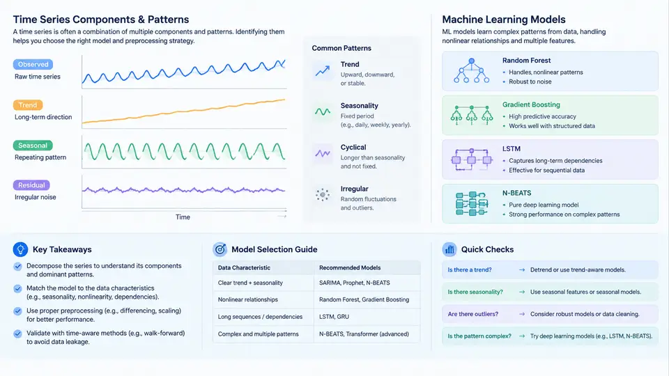
Time series forecasting is the task of predicting future values of a sequence of observations ordered in time. Unlike ordinary regression, where samples are assumed independent, a time series carries temporal dependence: today's value is often correlated with yesterday's, last week's, or the same hour in a previous season. This dependence is both the difficulty and the opportunity. A forecasting model must extract structure from the past and project it forward, while respecting the fact that the data-generating process can shift over time.
Before choosing any algorithm, it is essential to understand what a time series is made of. Classical decomposition separates an observed series y_t into interpretable components:
- Trend (Tt) — the long-term direction, such as steady growth in monthly electricity demand.
- Seasonality (St) — repeating patterns at a fixed period, such as daily traffic peaks or annual retail cycles.
- Cyclical component (Ct) — longer, non-fixed oscillations like economic expansions and recessions.
- Residual/irregular (Rt) — what remains after the structured components are removed, ideally close to white noise.
These components combine either additively (y_t = T_t + S_t + C_t + R_t) when the seasonal amplitude is roughly constant, or multiplicatively (y_t = T_t × S_t × C_t × R_t) when the amplitude grows with the level. Choosing the wrong form distorts the seasonal estimate, so a quick diagnostic is to plot the seasonal swing at low and high levels of the series: if the swing widens proportionally, prefer the multiplicative form.
Patterns That Drive Forecastability
Beyond decomposition, several pattern properties determine how hard a series is to forecast. Stationarity means the statistical properties (mean, variance, autocovariance) do not change over time. Many models, including ARIMA, assume weak stationarity and require differencing to achieve it. Autocorrelation measures how strongly a value depends on its own lags; the ACF and PACF plots reveal this structure. Seasonality strength and trend strength can be quantified, for example using the STL decomposition-based measures proposed by Hyndman, which help decide whether seasonal differencing is warranted.
Another critical property is heteroscedasticity — variance that changes over time. Financial returns often exhibit volatility clustering, where large changes follow large changes. Ignoring this leads to prediction intervals that are too narrow in turbulent periods. Finally, structural breaks (policy changes, pandemics, sensor recalibration) violate the assumption that the past resembles the future, and no purely statistical model can anticipate them without external regressors or human intervention.
Why Machine Learning Models Enter the Picture
Classical models such as ARIMA, Exponential Smoothing, and Theta are strong, interpretable baselines, especially for univariate series with clear linear structure. However, real-world forecasting increasingly involves conditions classical models handle poorly:
- High-dimensional exogenous inputs — weather, promotions, holidays, prices, and sensor readings that jointly influence the target.
- Nonlinear relationships — thresholds, interactions, and saturation effects that linear models cannot capture.
- Many related series — thousands of SKUs or sensors that share patterns and can borrow strength from one another (global models).
- Irregular or missing data — machine learning pipelines can incorporate imputation and masking more flexibly.
Machine learning reframes forecasting as supervised learning. Given a series, we construct a design matrix where each row is a feature vector at time t and the label is y_{t+h}. Features typically include lagged values (y_{t-1}, y_{t-2}, …, y_{t-p}), rolling statistics (mean, std, min, max over windows), calendar features (hour, day-of-week, month, holiday flags), and exogenous variables. Algorithms such as gradient-boosted trees (XGBoost, LightGBM), random forests, and neural networks (LSTM, Temporal Convolutional Networks, Transformers) then learn the mapping.
A Concrete Feature Construction Example
Suppose we forecast hourly bike-sharing demand. A minimal supervised framing with a 24-hour horizon looks like this:
import pandas as pd

# df: timestamp index, column 'demand'
df = df.sort_index()
df['lag_1']   = df['demand'].shift(1)
df['lag_24']  = df['demand'].shift(24)
df['lag_168'] = df['demand'].shift(168)          # one week
df['roll_mean_24'] = df['demand'].shift(1).rolling(24).mean()
df['roll_std_24']  = df['demand'].shift(1).rolling(24).std()
df['hour']    = df.index.hour
df['dow']     = df.index.dayofweek
df['is_weekend'] = (df['dow'] >= 5).astype(int)

# Target: demand 24 hours ahead
df['y'] = df['demand'].shift(-24)
df = df.dropna()
Note the deliberate use of shift(1) before rolling statistics. Without it, the rolling mean at time t would include y_t, leaking the target into the features and producing unrealistically optimistic validation scores. This data leakage is the most common and most damaging mistake in applied forecasting.
Validation Must Respect Time
Random k-fold cross-validation is invalid for time series because it trains on future data to predict the past. Instead, use rolling-origin or expanding-window backtesting: train on [0, t], validate on [t+1, t+h], then advance t and repeat. This mimics the real deployment condition where only past data is available at prediction time.
Choosing Between Classical and ML Approaches
The decision is not binary. A practical workflow starts with a strong classical baseline (e.g., seasonal naive, ETS, or ARIMA) to establish a reference error. If the ML model cannot beat that baseline on rolling-origin validation, the added complexity is unjustified. ML tends to win when exogenous drivers matter, when many series can be pooled into a global model, or when nonlinearity is pronounced. Classical models tend to win on short, clean, univariate series where interpretability and fast iteration dominate.
Common Pitfalls to Avoid Early
- Leakage through rolling features — always shift before rolling.
- Random train/test splits — use chronological splits only.
- Ignoring the forecast horizon — a model tuned for 1-step-ahead may degrade badly at 24 steps; validate at the actual deployment horizon.
- Overfitting to a single validation window — use multiple rolling origins and report the distribution of errors, not a single number.
- Forgetting to refit — as new data arrives, models must be retrained or updated; a stale model silently drifts.
With these fundamentals in place — understanding components, recognizing pattern properties, framing the problem as supervised learning, engineering leak-free features, and validating with rolling origins — you have the conceptual foundation needed to move into specific model families and their practical tuning in the chapters ahead.