1. Industrial prediction systems
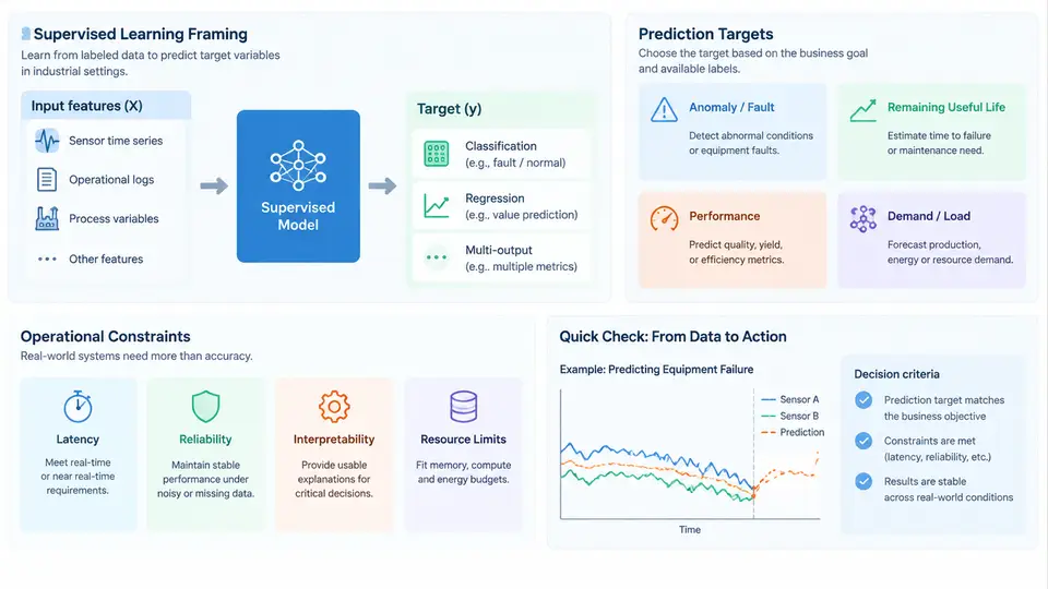
An industrial prediction system is not simply a model that produces a number. It is an engineered pipeline that maps sensor and process data to a decision-relevant quantity, and then delivers that quantity to a control room, a maintenance planner, or an automated controller within a time budget. Supervised learning provides the mathematical framing for this pipeline, but the framing only becomes useful when it is anchored to a concrete prediction target and a set of operational constraints that the model must respect in production.
Framing the Problem as Supervised Learning
In supervised learning, we assume a joint distribution over inputs X and targets Y, and we seek a function f: X → Y that minimizes expected loss on unseen data drawn from the same distribution. For industrial systems, X is typically a window of multivariate time-series measurements — temperatures, pressures, flow rates, vibration spectra, motor currents — and Y is a scalar or vector describing a future state or quality outcome.
The framing forces three explicit decisions that are often left implicit in academic exercises but are unavoidable in industry:
- What exactly is the target? A remaining useful life in hours, a binary fault flag, a continuous quality measurement, or a probability of failure within a horizon.
- What is the prediction horizon? Predicting a failure 30 seconds ahead supports a different control action than predicting it 30 days ahead.
- What loss function reflects the real cost? A missed fault and a false alarm rarely have symmetric costs.
These decisions are not modeling details; they determine whether the system is useful. A model with excellent RMSE on a target that nobody acts on is worthless.
Prediction Targets in Industrial Contexts
Industrial prediction targets fall into a few recurring families. Regression targets include remaining useful life (RUL), product quality variables such as thickness or tensile strength, and energy consumption. Classification targets include fault type, pass/fail quality gates, and anomaly presence. Probabilistic targets include the probability of failure within a horizon or a full predictive distribution over RUL.
The choice of target determines the label construction process, which is often the hardest part of an industrial project. For RUL, labels are typically derived from run-to-failure histories or from maintenance records with known intervention times. For quality prediction, labels come from laboratory measurements that may be delayed by hours or days relative to the process data. This label latency is a first-class constraint: it limits how quickly a model can be retrained and how tightly the training set can track current operating conditions.
Operational Constraints That Shape the Design
Operational constraints are the conditions under which the model must function. They are not optional refinements; they eliminate entire classes of solutions. The most common constraints in industrial prediction systems are:
| Constraint | Typical Requirement | Design Impact |
|---|---|---|
| Latency | Inference in < 100 ms for closed-loop control | Excludes large ensembles and deep sequence models at the edge |
| Data availability | Labels delayed by hours to weeks | Requires drift monitoring and delayed-label retraining strategies |
| Class imbalance | Faults may be < 0.1% of samples | Requires resampling, cost-sensitive loss, or anomaly-detection framing |
| Interpretability | Operators must trust and act on alerts | Favors feature attribution, rule extraction, or physics-informed features |
| Deployment environment | Edge PLC, on-premise server, or cloud | Constrains model size, runtime, and update frequency |
| Safety and regulatory | No autonomous action without human confirmation | Model output is advisory; decision logic is separate |
These constraints interact. A low-latency requirement pushes toward simpler models, which may reduce accuracy on rare faults, which in turn increases the importance of cost-sensitive evaluation. A safety requirement that keeps the model advisory changes the evaluation metric from raw accuracy to alert precision at a fixed recall, because operators will ignore a system that cries wolf.
From Framing to a Concrete Pipeline
A practical industrial prediction system can be organized as a sequence of stages, each with its own inputs, outputs, and failure modes. The diagram below shows the core data and decision flow, including the feedback loop from operational outcomes back into retraining.
The diagram makes two points explicit. First, the model is one stage among several; feature engineering and decision logic often determine field performance more than the choice of algorithm. Second, the feedback loop from outcomes to retraining is not instantaneous. Labels arrive late, and the system must remain safe and useful while the training distribution drifts.
Evaluation Under Operational Constraints
Standard cross-validation accuracy is rarely the right metric. In an industrial setting, evaluation should reflect the decision the model supports. For a fault alarm, the relevant quantities are precision at the operating threshold, recall at that threshold, and the expected cost per decision. For RUL regression, the relevant quantity may be the asymmetric cost of early versus late prediction, since predicting failure too late is usually far more expensive than predicting it too early.
A practical evaluation protocol includes:
- Temporal splits rather than random splits, so that the model is tested on future data relative to training.
- Cost-weighted metrics that encode the relative cost of false negatives and false positives.
- Drift checks comparing input feature distributions between training and deployment windows.
- Shadow mode deployment, where the model runs alongside the existing system without acting, to collect real-world performance before go-live.
Common Failure Modes at the Framing Stage
Many industrial prediction projects fail before modeling begins. The most frequent framing errors are:
- Target leakage: using a feature that is only available after the event being predicted, such as a maintenance log entry created when the fault was confirmed.
- Horizon mismatch: training on a 1-hour-ahead target but deploying where decisions are made 24 hours ahead.
- Ignoring label delay: assuming labels are available at the same time as features, which leads to over-optimistic offline metrics.
- Treating all errors as equal: optimizing accuracy when the cost of a missed fault is orders of magnitude higher than a false alarm.
- Neglecting the deployment environment: selecting a model that cannot run within the latency or memory budget of the target hardware.
Each of these errors is a framing error, not a modeling error. They are best caught by writing down the target, horizon, cost structure, and deployment constraints before any algorithm is selected. The remaining chapters build on this foundation: once the framing is correct, feature engineering, model selection, validation, and monitoring become tractable engineering tasks rather than open-ended research problems.