1. Course overview

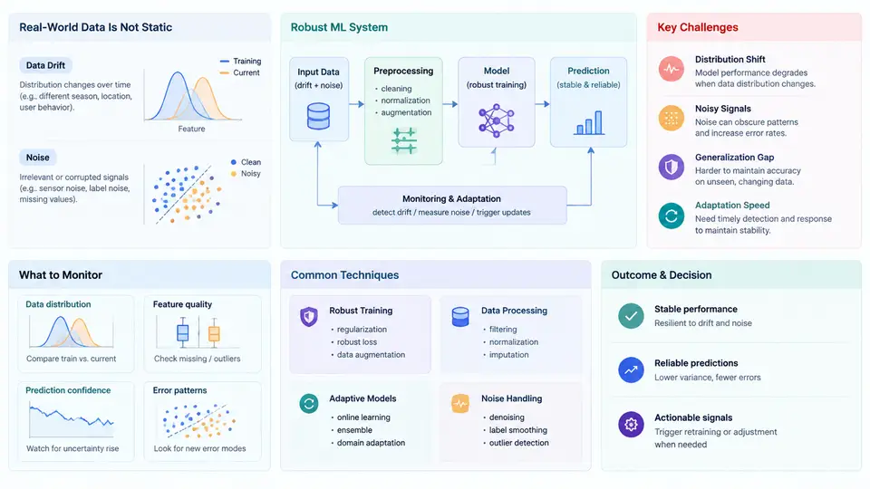
Production machine learning systems rarely operate on the clean, stationary distributions that dominate academic benchmarks. Once a model is deployed, the world it observes keeps moving: user behavior shifts, sensors age, upstream data pipelines change schema, and adversarial or accidental noise corrupts inputs. A model that achieved 0.94 AUC on a held-out test set can silently degrade to 0.71 within a quarter — often without any code change, alert, or crash. This course addresses that gap: how to design, train, monitor, and maintain machine learning systems whose predictive quality remains acceptable when the data distribution drifts and when inputs are noisy.

This first chapter establishes the vocabulary, the failure modes, and the technical context that the remaining 29 chapters build on. It is deliberately conceptual, but it is grounded in concrete signals and metrics you will use throughout the course.

What "Robustness" Means in This Course

Robustness is not a single property. In this course we treat it as a measurable, multi-dimensional target. A system is robust to the extent that it maintains specified performance under specified perturbations. That definition forces two questions that recur in every chapter: which perturbations, and how much performance loss is acceptable?

We distinguish four perturbation families that a deployed system must survive:

• Covariate shift — the input distribution P(X) changes while the conditional P(Y|X) stays roughly stable. Example: a fraud model trained on pre-holiday traffic sees a different transaction-amount distribution in December.
• Label / concept drift — the relationship P(Y|X) itself changes. Example: a credit-risk model where a macroeconomic shock alters default behavior for the same applicant profile.
• Feature noise — random or systematic corruption of individual inputs: sensor jitter, missing values, quantization, OCR errors, or adversarial perturbations.
• Label noise — incorrect training targets from annotation error, weak supervision, or feedback loops.

These are not independent. A noisy feature can look like covariate shift to a drift detector; a drifted label distribution can be misread as label noise. A recurring theme of this course is disambiguation: identifying which failure mode is actually occurring before choosing a remedy.

Why Standard ML Pipelines Fail

The canonical supervised pipeline — collect data, split into train/validation/test, fit, evaluate, deploy — embeds a stationarity assumption. The test set is drawn from the same distribution as training data, and it is evaluated once. Both assumptions break in production.

Three structural weaknesses follow:

1. Evaluation is a snapshot, not a process. A single held-out score cannot detect gradual drift. Robust systems require continuous evaluation against fresh, labeled data — or proxy metrics when labels are delayed.
2. Optimization targets average-case loss. Empirical risk minimization minimizes mean loss over the training distribution. It offers no guarantee on worst-case or shifted subpopulations, which is exactly where failures concentrate.
3. Monitoring is decoupled from modeling. Drift detection is often bolted on as an afterthought, so the model has no mechanism to adapt when drift is detected.

The Technical Landscape

The methods covered in this course fall into four layers, which also structure the syllabus. The diagram below shows how they connect: raw data flows through a training pipeline into a deployed model, while a parallel monitoring path observes live inputs and outcomes, and a feedback path triggers adaptation.

The four layers are: data (how distribution shift and noise enter the system), model (training objectives and architectures that tolerate perturbation), monitoring (detecting drift and estimating performance without fresh labels), and adaptation (retraining, reweighting, or online updates). Each layer has its own metrics and failure modes, and the course devotes multiple chapters to each.

Core Concepts and Notation

We use a consistent notation throughout. Let P₀(X, Y) denote the joint distribution at training time and Pₜ(X, Y) the distribution at deployment time t. A model f_θ maps inputs to predictions. The expected loss under the current distribution is:

L(t) = E_{(x,y) ~ Pₜ} [ ℓ(f_θ(x), y) ]

Robustness concerns the behavior of L(t) as Pₜ diverges from P₀. Two quantities matter in practice:

• Degradation — the increase L(t) − L(0). A robust system keeps this bounded.
• Detection latency — the number of time steps between the onset of drift and its detection. A robust system minimizes this, even if the model itself cannot adapt instantly.

For noise, we distinguish aleatoric noise (irreducible randomness in the data-generating process) from epistemic uncertainty (reducible with more data). This distinction determines whether more data helps or whether the model must be made inherently tolerant.

What You Will Build

By the end of the course you will be able to:

• Diagnose whether a performance drop is caused by covariate shift, concept drift, feature noise, or label noise, using distributional tests and error analysis.
• Select and implement drift detectors (Kolmogorov–Smirnov, Population Stability Index, Maximum Mean Discrepancy) and calibrate their thresholds against false-alarm rates.
• Train models with robustness-oriented objectives: importance weighting, distributionally robust optimization, and noise-robust losses.
• Estimate live performance when labels are delayed, using proxy signals and importance-weighted validation.
• Design a retraining and rollback policy that balances adaptation speed against stability.

How to Read This Course

Chapters 2–8 cover the data layer: characterizing drift, noise models, and the statistical tests that separate them. Chapters 9–18 cover the model layer: robust training objectives, regularization, ensembling, and uncertainty quantification. Chapters 19–25 cover monitoring: drift detection in practice, proxy metrics, and alerting design. Chapters 26–30 cover adaptation and system integration: retraining policies, online learning, and end-to-end case studies.

The central discipline of the course is measurement before remedy. Every chapter emphasizes how to observe the relevant signal — a distribution statistic, a loss curve, a calibration plot — and how to judge whether an intervention actually improved robustness. Without that discipline, robustness work becomes guesswork, and guesswork does not survive contact with production.