1. Engineering control systems as sequentia
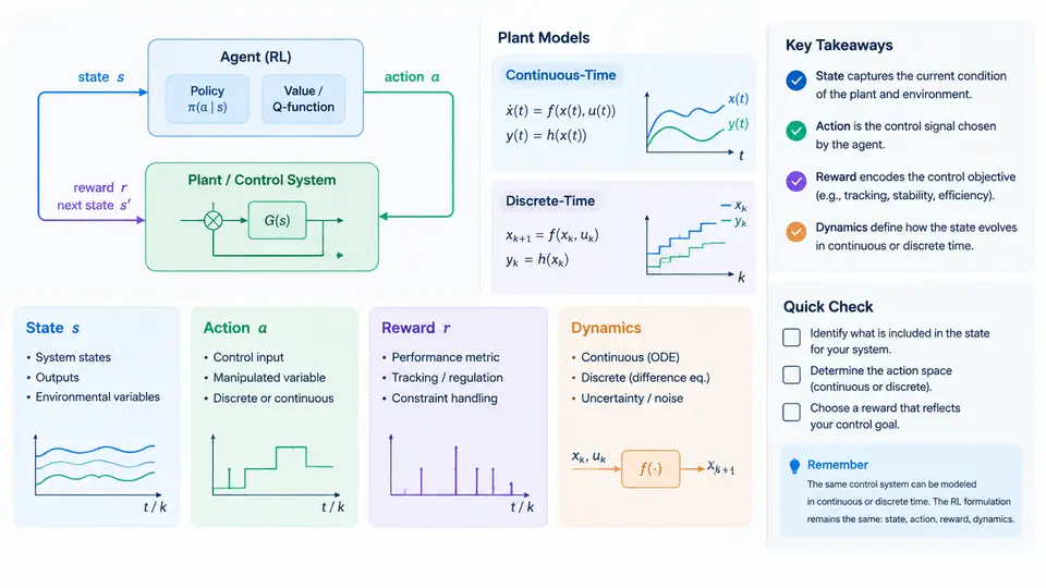
Every feedback controller is, at heart, a decision maker. At each instant it observes something about the plant, chooses a control input, and then lives with the consequences. Reinforcement learning (RL) formalizes exactly this loop, but it does so with a vocabulary — state, action, reward, dynamics — that must be mapped carefully onto the continuous-time and discrete-time plants that control engineers already know. This chapter builds that mapping. The goal is not to replace classical control intuition, but to express it in a form an RL agent can optimize.
1.1 The Control Loop as a Decision Process
Consider a plant described by a nonlinear ordinary differential equation:
ẋ(t) = f(x(t), u(t), t),   x(t₀) = x₀
y(t)  = g(x(t), u(t), t)
Here x ∈ ℝⁿ is the state, u ∈ ℝᵐ is the control input, and y is the measured output. In classical design we ask: find u(t) such that y tracks a reference while respecting actuator limits. In the RL formulation we ask a subtly different question: find a policy π that maps observations to actions so as to maximize a cumulative reward. The plant dynamics f become the transition model; the controller becomes the agent; the reference and constraints are folded into the reward.
The four canonical elements are:
- State
s— a sufficient statistic for predicting future behavior. For a plant, this is the physical state vector (positions, velocities, temperatures, currents), not merely the sensor reading. - Action
a— the control input applied over one decision interval. In continuous plants this is a held value (zero-order hold) or a parameterized waveform. - Reward
r— a scalar signal encoding task performance and constraint violations. - Dynamics
P(s′ | s, a)— the transition kernel, derived fromfand the sampling scheme.
1.2 Continuous-Time vs. Discrete-Time Plants
Physical plants evolve in continuous time, but digital controllers act at discrete instants. The bridge is the sampling period Δt. Under a zero-order hold, the continuous dynamics are discretized:
x[k+1] = x[k] + ∫ₖΔt^(k+1)Δt f(x(τ), u[k]) dτFor a linear time-invariant plant ẋ = Ax + Bu, this yields the exact discrete form x[k+1] = A_d x[k] + B_d u[k] with A_d = e^{AΔt} and B_d = (∫₀^Δt e^{Aτ} dτ) B. The choice of Δt is not cosmetic: it determines the effective action space, the reward accumulation, and whether the Markov property holds for the sampled state.
| Aspect | Continuous-time plant | Discrete-time MDP |
|---|---|---|
| Time | t ∈ ℝ | k ∈ ℕ |
| Transition | ẋ = f(x,u) | P(s′|s,a) |
| Action | Signal u(t) | Held value a[k] |
| Reward | Rate r(t) | Accumulated r[k] |
| Discounting | e^{-ρt} | γ^k |
The discount factors are related by γ = e^{-ρΔt}. This identity matters when transferring a continuous-time cost (e.g., a quadratic regulation cost) into a discrete RL objective: choosing γ independently of Δt silently changes the effective horizon.
1.3 Reward Design for Control Tasks
A control engineer's specification — settling time, overshoot, steady-state error, actuator effort — must be compressed into a scalar reward. A common and defensible choice is the negative of a stage cost:
r[k] = -( (x[k] - x_ref)ᵀ Q (x[k] - x_ref) + u[k]ᵀ R u[k] + penalty[k] )where Q ⪰ 0 and R ≻ 0 weight tracking error and control effort. Constraint violations (e.g., |u| > u_max, temperature above limit) are added as large negative penalties. The agent then maximizes Σ γᵏ r[k], which is the discrete analogue of minimizing an infinite-horizon LQR cost.
1.4 A Worked Example: DC Motor Speed Regulation
Take a brushed DC motor with armature resistance R_a = 1.2 Ω, inductance L_a = 5 mH, back-EMF constant K_e = 0.05 V·s/rad, torque constant K_t = 0.05 N·m/A, rotor inertia J = 2×10⁻⁴ kg·m², and viscous friction b = 1×10⁻⁴ N·m·s/rad. The state is x = [i, ω]ᵀ, the input is armature voltage u = V, and the output is speed ω.
di/dt = (V - R_a·i - K_e·ω) / L_a
dω/dt = (K_t·i - b·ω) / J
Discretize with Δt = 1 ms using the matrix exponential. The action is the voltage held over each millisecond, clipped to [-12 V, +12 V]. The reward uses Q = diag(0, 1) (penalize speed error only) and R = 0.01. A reference step from 0 to 100 rad/s is applied at t = 0.1 s.
To verify the discretization before any learning, simulate the discrete model against the continuous ODE with a fine solver. The two speed trajectories should agree to within a few percent over 0.5 s. If they diverge, the sampling period is too coarse relative to the electrical time constant L_a/R_a ≈ 4.2 ms — a classic sign that the discrete MDP is not a faithful representation of the plant.
τ_e = L_a/R_a and mechanical time constant τ_m = J/b differ by orders of magnitude. If Δt is chosen near τ_e, the current dynamics are aliased and the agent will learn a policy that works in simulation but fails on hardware.
1.5 The Markov Property and State Sufficiency
An RL agent assumes P(s′ | s, a) depends only on the current state. For a plant, this holds only if s contains all relevant physical variables. If the agent observes only ω but not i, the current is a hidden variable and the process is a partially observable MDP (POMDP). Two remedies are standard: (i) augment the observation with a short history of measurements, or (ii) use a recurrent policy that maintains an internal estimate of the hidden state. For the DC motor, including both i and ω restores the Markov property exactly.
1.6 Visualizing the Mapping
The diagram below summarizes how a physical control loop maps onto the RL decision process, including the discretization step that connects continuous-time dynamics to the discrete transition kernel.
1.7 Key Takeaways
- A control loop becomes an MDP once you fix the sampling period, define the state as a Markov-sufficient vector, and express the task as a scalar reward.
- Continuous-time dynamics and discrete-time transitions are linked by the zero-order hold; the discount factor and sampling period are coupled through
γ = e^{-ρΔt}. - Reward design is the translation of control specifications into an optimization objective. Dense stage costs derived from tracking error and control effort are the most reliable starting point.
- If the observed signal does not contain the full physical state, the problem is a POMDP and requires history augmentation or recurrent policies.
- Always validate the discretized model against the continuous plant before training; a mismatch in time constants will produce policies that do not transfer to hardware.