1. Production AI system landscape
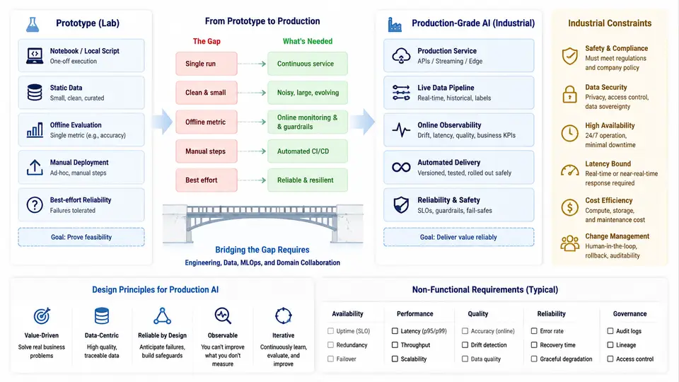
Most AI projects that succeed in a notebook never reach production. The gap is not primarily about model accuracy — it is about the engineering discipline required to keep a model correct, observable, and economically viable while it serves real traffic under real constraints. This chapter defines what "production-grade AI" actually means in industrial settings, catalogs the constraints that shape system design, and maps the specific failure modes that separate a demo from a deployable system.
What Makes an AI System "Production-Grade"
A production AI system is one that satisfies five properties simultaneously, not sequentially. A model that is accurate but unmonitored is not production-grade. A monitored model that costs $0.40 per inference on a $0.02-margin product is not production-grade either.
| Property | Prototype Standard | Production Standard |
|---|---|---|
| Correctness | Held-out accuracy on a static test set | Accuracy maintained across distribution shift, with drift detection and rollback |
| Latency | Batch inference, no deadline | p99 latency within the caller's timeout budget (e.g., ≤ 200 ms for inline APIs) |
| Availability | Runs when the developer runs it | Defined SLO (e.g., 99.9% monthly), graceful degradation on dependency failure |
| Cost | Ignored or measured per experiment | Bounded cost per request and per day, tracked against unit economics |
| Reproducibility | Random seed in a notebook cell | Versioned data, code, and model artifacts; any prediction traceable to a build |
The critical insight is that these properties interact. Reducing latency by shrinking the model may degrade accuracy below the SLO. Adding a fallback path improves availability but doubles the surface area to monitor. Production design is the practice of resolving these trade-offs explicitly rather than discovering them in an incident review.
Industrial Constraints That Shape the Design
Industrial deployments impose constraints that consumer-scale AI rarely faces. These are not edge cases; they are the design envelope.
- Deterministic timing. A vision inspection model on a conveyor running at 1.2 m/s has a hard per-frame budget. If inference takes 45 ms and the frame interval is 33 ms, the system drops frames regardless of accuracy. The latency budget is derived from the physical process, not from the model.
- On-premise or edge execution. Many plants prohibit outbound network calls for process data. This eliminates hosted API inference and forces quantization, pruning, or distillation to fit within the available accelerator memory (often 4–16 GB shared with other workloads).
- Regulatory traceability. In pharmaceutical or automotive contexts, every prediction that triggers an action must be logged with the model version, input hash, and timestamp. A model update without a corresponding audit record is a compliance failure, not just a bug.
- Long-tail failure cost asymmetry. A false negative in defect detection may ship a faulty part; a false positive stops the line. The cost ratio might be 100:1, which means the decision threshold is an economic parameter, not a default of 0.5.
- Data gravity and labeling latency. Ground truth may arrive hours or days after inference (e.g., after downstream QA). Online learning is usually infeasible; the system must operate on a delayed feedback loop.
The Prototype-to-Production Gap
The gap is best understood as a set of missing subsystems. A prototype typically contains only the model and a thin inference wrapper. A production system requires at least six additional concerns, each of which can independently block deployment.
The diagram above shows the subsystems that must exist around the model. The prototype contains only the two blue boxes on the left. Everything in the green region is additional engineering surface. The orange panel lists constraints that shape how each subsystem is built — for example, "on-prem only" forces the inference server to run locally and eliminates managed prediction APIs, while "regulatory audit trail" forces the audit log to be append-only and tamper-evident.
A Concrete Gap Analysis: Defect Detection Example
Consider a surface defect detection model for a steel rolling line. The prototype achieves 97.2% recall on a held-out set of 5,000 images. The team expects a smooth deployment. Here is what actually blocks it.
- Latency. The prototype runs at 120 ms per image on a workstation GPU. The line camera produces 30 frames per second, giving a 33 ms budget. The model must be quantized to INT8 and pruned, which drops recall to 94.1%. The team must decide whether 94.1% is acceptable or whether a two-stage approach (fast screening + slow confirmation on flagged frames) is needed.
- Threshold. The prototype uses 0.5. In production, a missed defect costs an estimated $2,400 in downstream rework, while a false alarm costs $18 in operator inspection time. The cost-optimal threshold is not 0.5 — it is closer to 0.15, which raises false positives by 4× but reduces expected cost per frame by 31%.
- Drift. The prototype was trained on images from one lighting configuration. The plant has three lighting zones. Without per-zone monitoring, recall in zone C silently drops to 81% within two weeks as lamp aging shifts the input distribution.
- Traceability. The customer requires that any rejected part be traceable to the model version and input image. The prototype logs nothing. Adding structured logging with image hashing and model version adds 8 ms per inference and requires a local append-only store.
- Fallback. When the GPU is preempted by another workload, the system must not stop the line. A CPU-based fallback model with lower accuracy but 200 ms latency keeps the line running with a "degraded" flag that routes all decisions to human review.
How to Use This Landscape
The remaining chapters of this course build out each subsystem in the diagram. The order is deliberate: data and feature infrastructure first, because train/serve skew is the most common source of silent production failure; then serving and decision layers, where latency and cost trade-offs are resolved; then observability and feedback, which close the loop; and finally the operational practices — versioning, rollback, incident response — that keep the system correct over time.
Before moving on, apply the gap analysis to your own project. For each of the six production subsystems in the diagram, write one sentence describing what exists today and one sentence describing what is missing. If more than two subsystems are entirely absent, the project is still a prototype regardless of its accuracy. That assessment is the starting point for everything that follows.