1. Industrial anomaly detection landscape
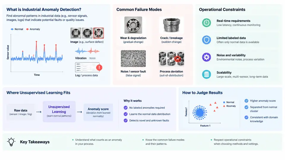
Industrial anomaly detection is the practice of deciding, from sensor and process data, whether a physical asset, product, or production run has departed from its normal operating behaviour. It sits at the intersection of condition monitoring, quality control, and machine learning, and it is defined less by the algorithm than by the operating environment: high cost of missed faults, extreme class imbalance, scarce labelled defects, and hard latency and false-alarm budgets. This chapter establishes the vocabulary, the failure modes we are trying to catch, the constraints that shape every design decision, and why unsupervised learning has become the default paradigm in this domain.
What Counts as an Anomaly
An anomaly is an observation that deviates from a well-defined notion of normality in a way that matters operationally. Three distinctions are worth fixing early, because they drive different detection strategies.
- Point anomalies — a single sample is abnormal in isolation, e.g. a vibration RMS reading of 12.4 mm/s on a bearing whose baseline is 1.8 mm/s.
- Contextual anomalies — a value is abnormal only given context, e.g. a mould temperature of 210 °C is normal during heating but abnormal during steady-state holding.
- Collective anomalies — an individual sample looks fine, but the sequence is wrong, e.g. a pressure curve that is smooth where it should show a characteristic step.
Equally important is the distinction between anomaly and fault. An anomaly is a statistical or behavioural deviation; a fault is a confirmed physical defect. Detection systems produce anomaly scores, not diagnoses. A high score means "this deserves inspection", and the inspection outcome is what closes the loop.
Failure Modes in Industrial Assets
Detection targets are usually grouped by degradation mechanism, because the mechanism determines which signals carry the earliest evidence.
| Failure mode | Typical asset | Leading indicator | Onset character |
|---|---|---|---|
| Bearing spalling / wear | Motors, fans, gearboxes | Envelope-spectrum energy at BPFO/BPFI | Gradual, weeks |
| Imbalance / misalignment | Rotating shafts | 1× and 2× running-speed amplitude | Step change after maintenance |
| Tool wear | CNC spindles, presses | Cutting force, spindle current, acoustic emission | Gradual, drift |
| Process drift | Reactors, extruders | Slow shifts in temperature/pressure setpoints | Very gradual |
| Leak / blockage | Pumps, valves, pipes | Flow–pressure relationship, differential pressure | Sudden or intermittent |
| Sensor fault | Any instrumented loop | Stuck value, flatline, out-of-range, rate-of-change | Sudden |
Sensor faults deserve explicit mention: they are anomalies in the data pipeline, not in the asset, and they are the single most common source of false positives. A stuck thermocouple produces a perfectly stable signal that any drift detector will eventually flag as "too normal".
Operational Constraints
Industrial deployments impose constraints that rarely appear in academic benchmarks.
- Class imbalance and label scarcity. A plant may run for years without a confirmed failure of a given type. Labelled defect sets are often in the tens of examples, while normal data is effectively unlimited.
- Asymmetric cost. A missed bearing failure can cost tens of thousands in collateral damage; a false alarm costs an inspection and erodes operator trust. The tolerable false-positive rate is often below 1 per asset per week.
- Latency and cadence. Vibration monitoring may run at 25.6 kHz, while a slow process loop samples at 1 Hz. Detection windows must match the physics, not the convenience of the model.
- Non-stationarity. Setpoints change with product grade, ambient temperature varies seasonally, and equipment is overhauled. A model trained on January data may be invalid by July.
- Edge and legacy integration. Inference frequently runs on a PLC-adjacent gateway or an IPC with limited memory, and results must reach SCADA or a historian via OPC UA, Modbus, or MQTT.
- Explainability and auditability. Maintenance engineers need to know which signal and which time window triggered an alert before they will act on it.
Why Unsupervised Learning Fits
Supervised classification requires examples of every failure mode, including modes that have not yet occurred. Unsupervised anomaly detection instead models p(x), the distribution of normal operation, and flags samples with low likelihood or large reconstruction error. This has three practical advantages: it can be trained on data collected before any failure occurs; it generalises to unseen fault types; and it degrades gracefully when a new failure mode appears, producing an alert rather than silently misclassifying.
The trade-off is that the model has no notion of severity or cause. It answers "is this unlike normal?" but not "what is wrong?" or "how urgent is it?". This is why unsupervised detectors are typically paired with a diagnostic layer — spectral analysis, rule-based thresholds, or a physics model — and with a human confirmation step.
From Raw Signal to Alert: A Reference Pipeline
The following SVG shows the canonical data path for an unsupervised industrial detector, from sensor acquisition through feature extraction, normal-behaviour modelling, scoring, and the decision layer that produces an operator-facing alert. It also marks the two points where the most common failure modes enter: sensor faults at acquisition, and threshold drift at the decision layer.
A Concrete Walkthrough
Consider a 7.5 kW centrifugal pump on a cooling loop, instrumented with a triaxial accelerometer on the drive-end bearing (25.6 kHz), motor current (1 kHz), and discharge pressure (1 Hz). The goal is early detection of bearing degradation without flooding the maintenance queue.
Inputs and baseline. Two weeks of data are collected during verified healthy operation, covering both duty points the pump actually runs at. Windows of 1 second with 50 % overlap yield roughly 1.2 million windows. For each window we compute RMS velocity, kurtosis, crest factor, and the envelope-spectrum amplitudes at the bearing defect frequencies BPFO and BPFI, derived from the shaft speed and bearing geometry.
Modelling. A PCA model is fitted on the standardised feature matrix, retaining components explaining 95 % of variance. The anomaly score for a new window is the squared reconstruction error, normalised by the 99th percentile of the training scores. This is deliberately simple: it is fast enough for edge inference, and its residuals can be traced back to individual features.
Decision layer. A raw score above 1.0 triggers a candidate; the alert is only raised if the score stays above threshold for 5 consecutive windows (5 seconds) and the BPFO amplitude itself exceeds its own baseline by 3σ. This persistence rule suppresses single-window spikes from electrical noise or a transient load change.
What to observe. In a healthy pump, the score fluctuates between 0.2 and 0.7 with occasional excursions during start-up. Early bearing wear typically appears as a slow upward trend in the BPFO feature while RMS remains flat — the score crosses 1.0 first, often days before the overall vibration level rises. A sudden score jump accompanied by a flatlined current signal indicates a sensor problem, not a mechanical one.
What This Course Builds Toward
The remaining chapters move from this landscape view into the mechanics: feature engineering for vibration and process signals, density- and reconstruction-based detectors, threshold selection under asymmetric cost, drift handling, and deployment on constrained hardware. The recurring theme is that in industrial settings the model is the easy part — the hard part is defining normal, keeping that definition current, and making alerts trustworthy enough that someone acts on them.