1. Industrial fault localization landscape
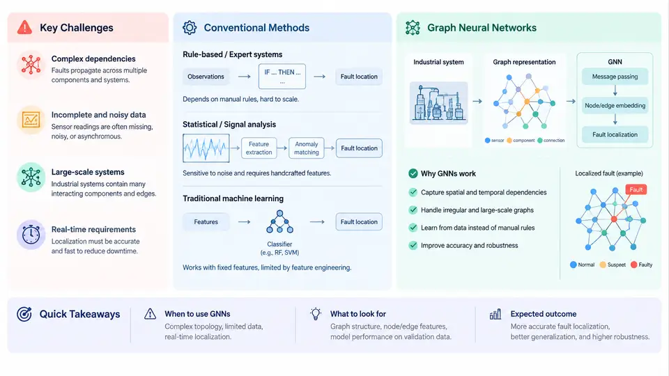
Fault localization is the task of determining where a fault originates in a system, as opposed to merely detecting that something is wrong. In industrial settings — process plants, power grids, manufacturing lines, rotating machinery fleets — this distinction matters enormously. A detection alarm tells an operator that a deviation exists; localization tells maintenance and control engineers which asset, subsystem, or sensor path to act on. The gap between the two is where most operational cost, downtime, and safety risk accumulates.
This chapter establishes the problem landscape: why industrial fault localization is structurally difficult, what conventional methods do well and where they break down, and why graph neural networks (GNNs) have become a natural fit for the topology-rich, sensor-dense systems found in modern industry.
Why Industrial Fault Localization Is Hard
Three properties of industrial systems make localization fundamentally harder than classification on a clean dataset.
Fault propagation and masking. A root-cause fault rarely stays local. A bearing degradation in a pump may raise vibration, change discharge pressure, and shift motor current — all of which propagate to neighboring units through shared headers, shafts, or electrical buses. Downstream sensors therefore report symptoms, not causes. Worse, propagation can mask the origin: a downstream anomaly may dominate the signal magnitude while the true root cause remains subtle.
Sensor topology is not a grid. Industrial instrumentation is deployed according to process connectivity, not spatial regularity. Two sensors physically adjacent on a skid may be hydraulically unrelated; two sensors far apart may be tightly coupled through a recycle loop. Any method that assumes Euclidean locality — as convolutional architectures do — is implicitly making a false assumption about the data.
Label scarcity and class imbalance. Genuine labeled fault events are rare, expensive to obtain, and often ambiguous even to domain experts. A plant may record thousands of normal operating hours for every confirmed root-cause event. Supervised localization models trained on such data overfit to the few fault classes they have seen and fail on novel combinations.
Conventional Methods and Their Limits
Conventional approaches fall into four broad families, each with a characteristic failure mode.
| Family | Representative technique | Strength | Primary limitation |
|---|---|---|---|
| Model-based | Observer / parity-space residual generation | Interpretable residuals, strong theory | Requires accurate first-principles model; degrades under unmodeled dynamics |
| Signal-based | Spectral analysis, envelope demodulation, wavelet features | Excellent for single-component diagnosis | Local by construction; cannot attribute across coupled units |
| Data-driven (flat) | PCA/T², autoencoders, 1D-CNN, LSTM classifiers | No physical model needed; scales to many tags | Treats tags as an unordered vector; ignores connectivity |
| Knowledge-based | Fault trees, expert rules, signed directed graphs | Encodes causal expertise; auditable | Brittle, manual to maintain, poor at continuous-valued evidence |
The common thread in the limitations is structure loss. Model-based and signal-based methods are strong but local. Flat data-driven methods are scalable but permutation-invariant — they would produce identical outputs if you shuffled the sensor columns, which is clearly wrong for a plant. Knowledge-based methods encode structure but cannot learn from data.
Consider a concrete example. A three-unit compressor train has 24 vibration tags, 6 temperature tags, and 4 pressure tags. A PCA-based residual detector flags high T² at tags on Unit 2 and Unit 3 simultaneously. A flat classifier must learn, from data alone, that Unit 2's tags are upstream of Unit 3's and that the shared coupling is the interstage cooler. With limited fault labels, it usually cannot. A method that knows the coupling graph can propagate evidence along it directly.
What GNNs Bring to the Problem
A graph neural network operates on a graph G = (V, E) where nodes V carry feature vectors and edges E encode relationships. In industrial fault localization, the mapping is natural:
- Nodes = sensors, actuators, assets, or control loops, each with a time-windowed feature vector (RMS, kurtosis, spectral centroid, residual statistics).
- Edges = physical connectivity (piping, shaft, bus), causal influence, or learned statistical dependency.
- Node labels = fault/no-fault, or root-cause class for localization.
Message passing lets each node aggregate information from its neighbors. After k layers, a node's representation reflects its k-hop neighborhood. This is exactly the propagation behavior that makes faults hard — and GNNs turn it from a nuisance into a modeling asset. A fault at a root node influences its neighbors' representations, and the network can learn to attribute the pattern back to the source.
Three properties make GNNs particularly suitable:
- Topology awareness. Predictions respect the actual coupling structure rather than an assumed grid.
- Inductive generalization. Because parameters are shared across edges, a GNN trained on one section of a plant can be applied to a structurally similar section with different tag counts.
- Interpretability hooks. Attention weights or edge gradients can be inspected to see which connections drove a localization decision — valuable for operator trust and for validating against P&IDs.
From Detection to Localization: A Reference Pipeline
The figure below shows how the pieces connect. Raw tags are windowed into features, the plant topology is assembled into a graph, and a message-passing network produces per-node fault scores that are then thresholded and ranked to yield a localized root cause.
What to Watch For
Two practical cautions belong in any first encounter with GNN-based localization.
Graph quality dominates model quality. If the edge set is wrong — missing a real coupling or asserting a spurious one — message passing will confidently propagate evidence in the wrong direction. Graph construction from P&IDs, historian correlation, or transfer-entropy estimates deserves as much engineering effort as architecture selection.
Evaluation must be localization-aware. Top-1 accuracy on a balanced test set is misleading. Report metrics that reflect operational reality: top-k hit rate at the true root-cause node, mean rank of the correct node, and false-localization rate under normal operation. A model that detects faults well but localizes them poorly is not solving this problem.
The remainder of this course builds on this foundation: constructing industrial graphs from real plant data, choosing message-passing architectures suited to continuous sensor features, training under label scarcity, and validating localization against known fault events. The central idea to carry forward is that industrial fault localization is a structured inference problem, and GNNs are the first mainstream family of models whose inductive bias matches that structure.