1. Industrial inspection landscape
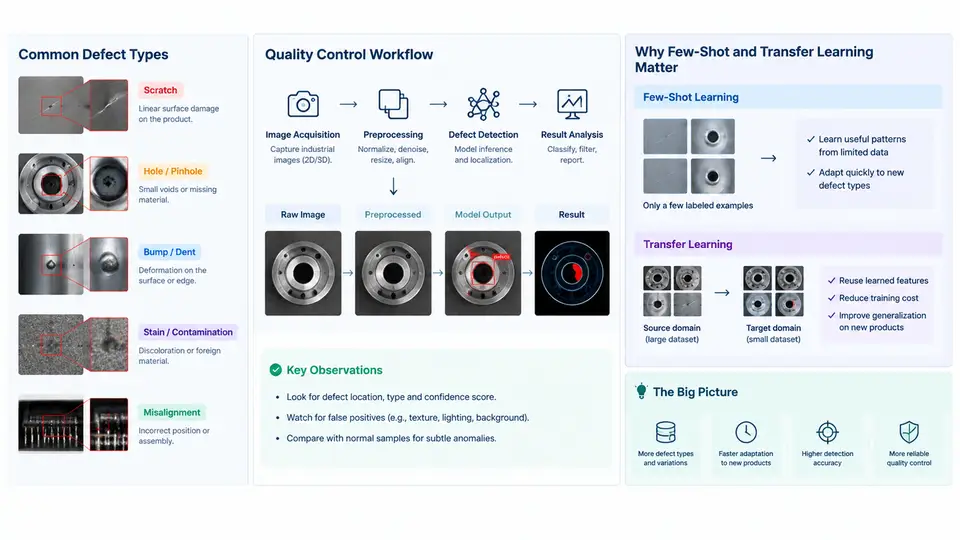
Industrial visual inspection is the task of deciding, from images or signals, whether a manufactured part meets its specification. That decision sounds simple, but the operating environment is hostile to conventional machine learning: defects are rare, their appearance drifts with every process change, and the cost of a missed escape is measured in recalls rather than accuracy points. This chapter maps the problem space — what defects actually look like, how inspection is embedded in production, and why few-shot and transfer learning have become the default engineering answer rather than an academic curiosity.
1.1 What "Defect" Actually Means on a Line
Defect taxonomy drives everything downstream: annotation strategy, model architecture, augmentation policy, and the acceptance threshold. In practice, inspection engineers group defects by their geometric and statistical signature rather than by their physical cause.
| Defect class | Typical signature | Detection difficulty | Common modality |
|---|---|---|---|
| Scratch / abrasion | Elongated, low-contrast, orientation-variable | High — blends with texture | Bright-field, dark-field |
| Dent / deformation | Local gradient change, shading shift | Medium — needs 3D or photometric cues | Structured light, photometric stereo |
| Contamination / foreign material | High-contrast blob, arbitrary shape | Low–medium | Color imaging |
| Missing / misplaced component | Presence–absence, positional offset | Low — structured | Area scan, template matching |
| Solder void / crack | Sub-surface, low SNR | Very high | X-ray, AXI, acoustic |
| Coating / print irregularity | Periodic texture deviation | High — statistical, not local | Line scan, spectral |
Two properties of this table matter more than the individual rows. First, the classes are not equally represented: a mature line may produce thousands of good parts per defect. Second, several classes are defined by deviation from a normal appearance rather than by a positive visual signature — a scratch is "not the surrounding texture," a void is "not the expected density." This asymmetry is the root cause of the data problem that few-shot learning addresses.
1.2 The Quality Control Workflow
Inspection is not a single model; it is a pipeline with distinct decision points, each with its own latency, recall, and cost budget.
- Acquisition. Trigger, illumination, exposure, and focus are fixed per part type. A change in lighting angle can move a defect from detectable to invisible without any change to the part.
- Pre-processing. Flat-field correction, distortion removal, ROI extraction, and normalization. This stage is where most "the model stopped working" incidents actually originate.
- Detection / segmentation. Localize candidate defects. High recall is prioritized here; false positives are tolerated because they are filtered later.
- Classification. Assign a defect type and severity to each candidate. This is where precision matters and where few-shot methods are most valuable.
- Disposition. Accept, reject, or route to human review, governed by an acceptance threshold and a cost model.
- Feedback. Escapes and over-kills are fed back as new labeled examples — the loop that keeps the system alive.
1.3 Why Few-Shot and Transfer Learning Matter
Consider a realistic commissioning scenario. A new product variant enters a line that already inspects three similar variants. The customer supplies 15 labeled defect images across 4 defect classes, plus roughly 200 defect-free images. A from-scratch CNN has no chance: 15 examples cannot constrain millions of parameters, and the resulting model will memorize rather than generalize.
Three forces make this the normal case rather than an edge case:
- Label scarcity. Defects are rare by definition. Collecting 1,000 examples of a specific scratch type may take months of production.
- Distribution shift. Tooling wear, material lot changes, and seasonal humidity alter image statistics continuously. A model trained on January data degrades by March.
- Long-tail class structure. A typical line has 3–5 frequent defect types and 20+ rare ones. The rare ones are the expensive ones.
Transfer learning addresses the first and third forces by reusing representations learned on large source datasets (ImageNet, COCO, or an in-house corpus of millions of industrial images). Few-shot learning addresses the second by making adaptation cheap: instead of retraining, the system conditions on a small support set at inference time.
1.4 A Concrete Commissioning Example
The following example illustrates the workflow and the parameters that matter. It is a representative setup, not a measured result.
Task: classify 4 defect types on stamped metal brackets
Support set: 15 labeled images (4 classes, 3-4 images each)
Query set: 120 unlabeled images from the current shift
Backbone: ResNet-18 pretrained on ImageNet
Method: prototypical network, 5-way 1-shot evaluation

Pre-processing:
  - flat-field correction with per-lens calibration frame
  - ROI crop to bracket face (fixed coordinates per fixture)
  - resize to 224x224, ImageNet normalization

Training:
  - freeze first two stages, fine-tune stages 3-4
  - lr = 1e-4, 200 episodes, 5-way 5-shot
  - augmentation: rotation +/-15 deg, brightness +/-10%

Inference:
  - compute class prototypes from support embeddings
  - assign query to nearest prototype (cosine distance)
  - threshold: reject if max similarity < 0.62
What to observe: the similarity distribution for known defect classes should be bimodal (clear separation between correct and incorrect assignments). If it is unimodal, the support set is too small or the backbone is mismatched to the modality. A common failure symptom is that all queries collapse to one prototype — usually caused by insufficient fine-tuning or by a support set where one class dominates.
1.5 The Inspection Decision Space
The figure below summarizes how defect characteristics, data availability, and method choice relate. It is not a flowchart to be executed step by step; it is a map of the trade-offs that determine which approach is appropriate for a given inspection task.
1.6 What This Course Covers
The remaining chapters build on this landscape. You will work through transfer learning fundamentals (feature extraction, fine-tuning schedules, domain adaptation), few-shot methods (prototypical networks, matching networks, MAML-style meta-learning), anomaly detection as the zero-label complement, and the engineering discipline of deploying and maintaining these systems on a live line. Each chapter includes concrete parameters, failure modes, and verification criteria so that the material can be reproduced on real inspection data.
The central engineering message of this chapter is that few-shot and transfer learning are not alternatives to classical inspection — they are the tools that make classical inspection viable when defect examples are scarce and the cost of a miss is high. The next chapter begins with the mechanics of transfer learning: what a pretrained backbone actually encodes, and how to decide which layers to freeze, fine-tune, or discard.