1. Industrial sensor data landscape
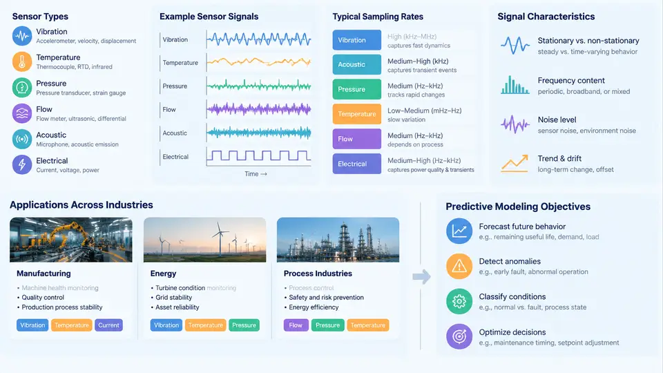
Predictive modeling for industrial systems begins long before the first model is trained. It begins with understanding what the sensors actually measure, how often they report, what their signals look like in both healthy and degraded states, and what decision the model is ultimately expected to support. A model that predicts the remaining useful life of a bearing and a model that flags an out-of-spec batch in a chemical reactor may share algorithms, but they consume fundamentally different data and answer fundamentally different questions. This chapter maps that landscape across manufacturing, energy, and process industries.
Sensor Types and What They Physically Measure
Industrial sensors fall into a few broad families, each with distinct signal behavior and modeling implications.
- Vibration (accelerometers, velocity transducers): mounted on rotating machinery such as motors, pumps, gearboxes, and turbines. They capture high-frequency oscillation, typically 1–50 kHz sampling, and are the primary source for bearing fault detection and imbalance diagnosis.
- Temperature (RTDs, thermocouples, thermistors): slow-moving signals, often sampled at 1 Hz or slower. Useful for detecting overheating, lubrication failure, and thermal drift, but rarely informative at high frequency.
- Pressure (piezoresistive, piezoelectric, differential): common in hydraulics, compressors, and process lines. Sampling ranges from 10 Hz to several kHz depending on whether transient surges matter.
- Flow (coriolis, ultrasonic, turbine): central to process industries; sampling is usually 1–10 Hz and signals are smooth but sensitive to fouling and calibration drift.
- Current and voltage (CTs, Hall-effect sensors): used for motor health, load estimation, and power quality. Motor current signature analysis (MCSA) exploits sidebands around the supply frequency to detect rotor faults.
- Acoustic emission and ultrasound: high-frequency, low-amplitude signals used for leak detection and early-stage crack propagation.
- Position, proximity, and encoders: provide timing and phase references that let other signals be angle-resolved rather than purely time-resolved.
The choice of sensor family constrains everything downstream: the sampling rate determines the Nyquist limit, the physical principle determines the noise model, and the mounting location determines how much attenuation and interference the signal accumulates before digitization.
Sampling Rates and the Information They Preserve
Sampling rate is not a convenience parameter — it defines which physical phenomena are even observable. A temperature channel sampled at 0.1 Hz cannot reveal a bearing defect whose characteristic frequency is 3.2 kHz. Conversely, storing 50 kHz vibration continuously for hundreds of channels produces terabytes per month and is rarely justified.
A practical rule is to sample at least 2.56× the highest frequency of interest (the Nyquist rate plus anti-aliasing margin). For envelope-based bearing analysis, this often means sampling at 20–50 kHz even though the fault frequencies of interest are below 500 Hz, because the resonance that the fault excites sits much higher. For slow process variables, 1 Hz is generous.
| Signal | Typical sampling rate | Primary modeling use |
|---|---|---|
| Bearing vibration | 20–50 kHz | Fault frequency detection, envelope analysis |
| Motor current | 5–20 kHz | Rotor bar and stator fault detection |
| Process pressure | 10–100 Hz | Surge, cavitation, control loop diagnosis |
| Temperature | 0.1–1 Hz | Thermal trend, overload detection |
| Flow | 1–10 Hz | Mass balance, fouling, leak detection |
Signal Characteristics That Shape Modeling Choices
Industrial signals are rarely clean. Three characteristics dominate practical work:
Non-stationarity. Load, speed, and ambient conditions change constantly. A vibration spectrum captured at 1500 rpm looks nothing like one captured at 900 rpm. Models must either normalize for operating condition or be trained across the full operating envelope.
Noise and interference. Electromagnetic interference from variable-frequency drives, ground loops, and sensor cable routing all inject artifacts. Distinguishing a genuine 60 Hz harmonic from a drive-induced one requires knowing the electrical environment, not just the signal.
Fault signatures buried in broadband content. A developing bearing defect may contribute less than 1% of total signal energy. Time-domain RMS alone will not reveal it; envelope demodulation, spectral kurtosis, or cepstral methods are needed to extract the signature.
Predictive Modeling Objectives by Industry
The same sensor infrastructure supports different prediction targets depending on the industry and the cost of failure.
In manufacturing, the dominant objectives are remaining useful life (RUL) estimation for rotating equipment, anomaly detection on assembly lines, and quality prediction from process signals. A stamping press monitored with accelerometers and current sensors might be modeled to predict tool wear, where the target is the number of strokes remaining before dimensional drift exceeds tolerance.
In energy, objectives include wind turbine gearbox failure prediction, transformer dissolved-gas trend forecasting, and grid asset health scoring. Here the cost of unplanned downtime is extreme, so models often prioritize recall over precision — missing a fault is far worse than a false alarm.
In process industries (chemicals, refining, pharmaceuticals), the focus shifts to soft sensing — inferring unmeasured quality variables from correlated measurements — and to early detection of process drift. A distillation column may have hundreds of temperature and pressure tags but only periodic laboratory samples of product purity; the model's job is to estimate purity continuously and flag deviations.
From Landscape to Modeling Decisions
The practical consequence of this landscape is that sensor selection and sampling design are modeling decisions, not just instrumentation decisions. Before writing any code, answer four questions:
- What is the prediction target, and what is its time horizon? RUL in hours, quality in the next batch, or anomaly within the next minute — each demands different feature windows and label definitions.
- What is the highest frequency that carries information about that target? This sets the minimum sampling rate and the feature extraction method.
- What operating conditions will the model see? If speed and load vary, the model needs condition normalization or condition-aware training.
- What is the cost asymmetry between false positives and false negatives? This determines the decision threshold and the evaluation metric long before training begins.
With this landscape established, the next step is to examine how raw signals become features — the transformation that turns high-rate waveforms and slow process trends into inputs a model can actually learn from.