1. Edge AI deployment landscape

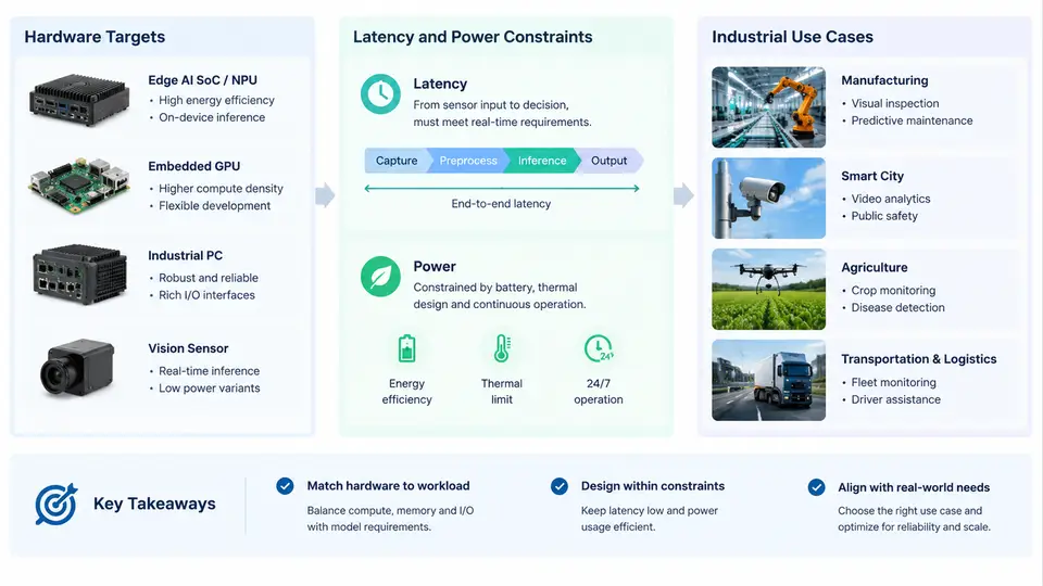
Edge AI deployment is not a single engineering problem but a multi-dimensional optimization problem. A model that runs comfortably on a cloud GPU may be entirely infeasible on a battery-powered industrial sensor, and a model that meets a 5 ms control-loop deadline on a mid-range SoC may exceed the thermal budget of a sealed enclosure. Before selecting a quantization scheme, a pruning ratio, or a runtime, you must first understand the deployment landscape: what hardware targets exist, what latency and power constraints they impose, and which industrial use cases drive those constraints.

Hardware Targets: A Tiered Landscape

Edge AI hardware is best understood as a tiered spectrum rather than a single category. Each tier has distinct compute characteristics, memory architectures, and power envelopes.

Tier	Representative Hardware	Typical Compute	Power Envelope	Typical Deployment
Microcontroller (MCU)	ARM Cortex-M4/M7, ESP32-S3, STM32H7	No NPU; DSP extensions, 100–480 MHz	10–500 mW	Keyword spotting, anomaly detection, vibration monitoring
Embedded CPU / low-power SoC	Raspberry Pi 4/5, Rockchip RK3399	Quad-core ARM, 1–2 TOPS NPU (optional)	2–10 W	Vision inspection, smart cameras, gateway inference
Edge accelerator	NVIDIA Jetson Orin Nano/NX, Google Coral, Hailo-8	10–275 TOPS INT8	5–25 W	Multi-camera perception, autonomous mobile robots, real-time video analytics
Industrial edge server	Intel Xeon + Flex GPU, AMD EPYC + Instinct	100+ TOPS, full FP16/INT8 support	50–300 W	Multi-line inspection, digital twin, on-premise training/fine-tuning

The key insight is that the hardware tier determines the feasible model architecture, precision, and runtime. An MCU with 512 KB SRAM cannot host a ResNet-50 in FP32; it requires aggressive quantization (INT8 or even binary) and a model whose peak activation memory fits within the SRAM budget. Conversely, a Jetson Orin NX can run a quantized YOLOv8 at 30 FPS with room for multi-model pipelines.

Latency Constraints: From Soft to Hard Real-Time

Latency in edge AI is not a single number. It decomposes into sensor acquisition, preprocessing, inference, postprocessing, and actuation. The end-to-end latency budget is what matters, and it is dictated by the control loop or decision cycle of the industrial process.

• Hard real-time (< 10 ms): Motor control, safety interlocks, high-speed sorting. Missing a deadline causes physical damage or safety hazards. These systems typically run on MCUs or FPGAs with deterministic execution, and the AI model is often a small classifier or anomaly detector.
• Firm real-time (10–100 ms): Robotic manipulation, autonomous navigation, quality inspection on moving production lines. Occasional deadline misses degrade quality but do not cause immediate failure. Edge accelerators like Jetson or Hailo are common here.
• Soft real-time (100 ms–1 s): Predictive maintenance, video analytics, human behavior monitoring. Latency affects user experience or throughput but not safety. Embedded CPUs and low-power SoCs suffice.
• Best-effort (> 1 s): Batch analytics, overnight model updates, non-critical logging. Cloud or industrial edge servers are acceptable.

When designing for a latency target, you must measure the full pipeline, not just the inference kernel. A model that infers in 8 ms but spends 15 ms on JPEG decode and 5 ms on NMS will miss a 20 ms deadline. Profiling tools such as nsys on Jetson, perf on Linux, or vendor-specific SDK profilers are essential.

Power Constraints: Thermal, Battery, and Cost

Power constraints manifest in three ways: thermal dissipation, battery life, and energy cost. In sealed industrial enclosures, the thermal design power (TDP) of the compute module determines whether active cooling is required. A fanless design typically limits sustained power to 5–15 W; exceeding this causes thermal throttling, which increases latency and variance.

For battery-powered devices, energy per inference is the critical metric. Consider a vibration sensor running an anomaly detection model every 100 ms. If the MCU consumes 50 mW active and 5 µW in sleep, and inference takes 2 ms, the average power is approximately:

P_avg = (P_active × t_active + P_sleep × t_sleep) / (t_active + t_sleep)
      = (50 mW × 2 ms + 0.005 mW × 98 ms) / 100 ms
      ≈ 1.005 mW

This yields years of battery life on a coin cell. But if the same model runs on a Jetson Orin Nano at 10 W, the battery lasts hours. The hardware tier and the duty cycle together determine feasibility.

Industrial Use Cases and Their Deployment Profiles

Different industrial use cases impose different combinations of hardware, latency, and power constraints. The following SVG maps four representative use cases to their deployment profiles, showing how the same AI capability (e.g., visual inspection) shifts across tiers depending on the required throughput and environmental constraints.

The table and diagram together reveal a critical engineering principle: the deployment target must be selected before model optimization begins. If you know the target is an MCU with 512 KB SRAM and a 10 mW average power budget, you immediately rule out FP32 models, large vision transformers, and any architecture requiring more than a few hundred kilobytes of activation memory. If the target is a Jetson Orin NX with a 25 W thermal design and a 20 ms latency budget, you have room for INT8-quantized convolutional networks but must still respect the memory bandwidth ceiling.

From Landscape to Optimization Strategy

Understanding the landscape directly informs the optimization strategy. For MCU-class targets, the priority is model compression: aggressive quantization (INT8, INT4, or binary), pruning, and knowledge distillation to fit within SRAM and flash constraints. For embedded SoC targets, the priority is runtime efficiency: selecting a runtime that exploits NEON or NPU instructions, optimizing preprocessing to avoid CPU-bound bottlenecks, and managing thermal throttling. For edge accelerator targets, the priority is throughput and batching: maximizing utilization of the NPU or GPU, overlapping data transfer with compute, and balancing multiple models in a pipeline. For industrial edge servers, the priority shifts to scalability and model freshness: supporting multiple concurrent inference streams, enabling on-premise fine-tuning, and managing model versioning across a fleet.

In the chapters that follow, each optimization technique—quantization, pruning, knowledge distillation, neural architecture search, and runtime-specific tuning—will be presented in the context of these deployment profiles. The goal is not to master a single technique in isolation but to build the judgment to select and combine techniques that satisfy the constraints of a given edge AI deployment.