1. Inspection system architecture
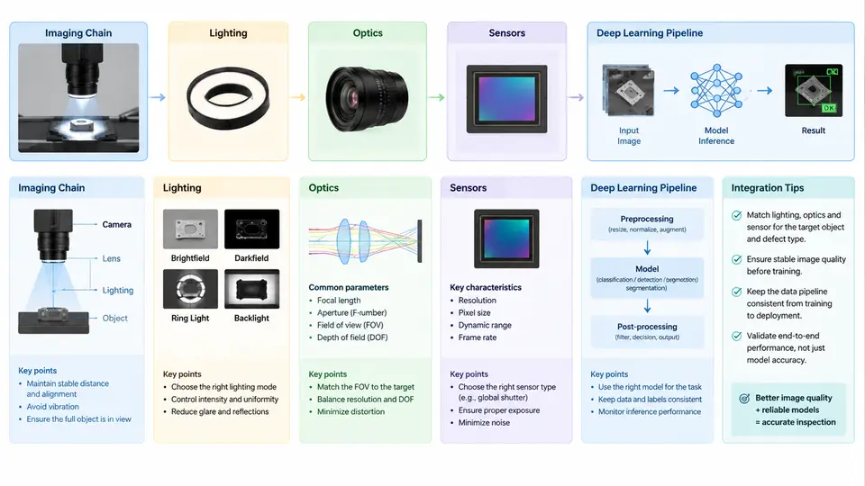
A machine vision inspection system is not a camera bolted to a conveyor with a neural network attached. It is a signal chain in which every stage transforms the physical state of a part into a decision. The architecture of that chain determines the ceiling of achievable accuracy: no model, however deep, can recover information that the optics never resolved or the lighting never revealed. This chapter establishes the end-to-end architecture and the engineering reasoning behind each interface.
The Imaging Chain as a Signal Path
The imaging chain converts a physical property of the inspected object — reflectance, geometry, transmission, or emitted radiation — into a digital array, then into a decision. The canonical stages are:
- Illumination — conditions the object so the defect of interest produces contrast.
- Optics — collects scattered or transmitted light and forms an image on the sensor plane.
- Sensor — converts photon flux to electrons and then to digital counts.
- Preprocessing — flat-field correction, dark offset subtraction, ROI extraction, and normalization.
- Deep learning inference — detection, segmentation, or classification producing defect maps and scores.
- Decision and actuation — thresholding, spatial aggregation, and reject/accept signaling to the PLC.
Each stage has a transfer characteristic. The system's contrast-to-noise ratio (CNR) at the defect is the product of the modulation each stage passes. Treating the chain as a cascade makes debugging tractable: when a defect is missed, you localize the loss by measuring the signal at each stage rather than retraining blindly.
Lighting: Engineering Contrast, Not Brightness
Lighting is the most under-engineered and highest-leverage stage. The goal is not illumination but selective contrast: making the defect differ from its background in the acquired image.
Common geometries and their appropriate use:
- Bright-field (direct) illumination — light coaxial with the camera axis. Good for surface print, matte defects, and general inspection. Specular surfaces produce glare that can mask defects.
- Dark-field illumination — light at a low grazing angle, camera off-axis. Only scattering features (scratches, edge chips, particles) appear bright against a dark background. Excellent for detecting surface micro-defects on polished parts.
- Backlight / transmitted illumination — light behind the part, camera in front. Produces a silhouette for dimensional measurement, hole presence, and edge position. Requires the part to be at least partially transmissive or the feature to be a through-hole.
- Diffuse dome illumination — a hemispherical diffuser surrounds the part. Produces uniform, shadow-free illumination for curved or specular parts where glare must be suppressed.
- Structured light / pattern projection — projects a known pattern to recover 3D shape via triangulation, used for height, warpage, and 3D defect detection.
Wavelength selection is a second lever. Because many materials have wavelength-dependent reflectance, a bandpass filter matched to the illumination LED (e.g., 630 nm red or 470 nm blue) can suppress ambient light and increase contrast between materials. For example, a red LED with a red bandpass filter makes a red label appear bright and a blue label dark, separating them without any software.
Optics: Resolution, Field of View, and Depth of Field
The optics determine the spatial sampling of the object. The governing relation for a lens of focal length f at working distance WD imaging a sensor of pixel pitch p is the object-space pixel size:
object_pixel_size = p * WD / f        (approximately, for WD >> f)

Example: p = 3.45 µm, WD = 300 mm, f = 25 mm
object_pixel_size = 3.45 µm * 300 / 25 = 41.4 µm/pixel

Field of view for a 2448 x 2048 sensor:
FOV_x = 2448 * 41.4 µm = 101.3 mm
FOV_y = 2048 * 41.4 µm = 84.8 mm
For reliable detection, the Nyquist criterion requires at least two pixels across the smallest feature, and industrial practice typically targets 3–5 pixels per defect dimension to preserve shape information for a CNN. A 0.1 mm defect therefore needs an object pixel size of roughly 20–33 µm.
Depth of field (DOF) must accommodate part height variation and fixturing tolerance. DOF shrinks with larger aperture (smaller f-number) and with higher magnification. If the part presents ±2 mm of height variation, either stop down (accepting less light and more diffraction), use a telecentric lens to remove perspective and magnification change, or add a focus-scanning mechanism.
Telecentric lenses are standard for dimensional metrology because they provide constant magnification across the field and a large DOF, eliminating perspective error on features away from the optical axis.
Sensors: Matching the Detector to the Task
| Sensor type | Strength | Typical inspection use |
|---|---|---|
| CMOS global shutter | No motion distortion, high frame rate | Moving parts on a conveyor, high-speed sorting |
| CMOS rolling shutter | Lower cost, higher resolution | Static or slow-moving parts |
| CCD | High uniformity, low noise | Legacy lines, low-light metrology |
| Line-scan | Very high resolution across a moving web | Web, sheet, and cylindrical surface inspection |
| InGaAs / SWIR | Sensitivity beyond 1000 nm | Moisture, subsurface, and through-plastic inspection |
| 3D (laser triangulation, ToF, structured light) | Height and volume | Warpage, solder joint volume, gap and flush |
Key sensor parameters to specify: quantum efficiency at the illumination wavelength, full-well capacity (dynamic range), read noise, dark current, and pixel pitch. A sensor with high quantum efficiency at 850 nm paired with an 850 nm LED will outperform a generic sensor under the same illumination.
Integrating the Deep Learning Pipeline
The deep learning stage consumes the preprocessed image and produces a defect map or classification. Integration decisions that matter architecturally:
- Where inference runs. Edge (on-camera or industrial PC with GPU) versus server. Edge inference keeps latency low and avoids network dependency; server inference centralizes model updates but adds jitter.
- Input contract. The model expects a fixed tensor shape, normalization, and color space. The preprocessing stage must guarantee this contract; a mismatch between training and inference normalization is a common silent failure.
- Output contract. Detection boxes, segmentation masks, or class scores must be converted to a pass/fail decision with a defined threshold and spatial aggregation rule (e.g., any defect pixel above score 0.5 within the ROI triggers reject).
- Latency budget. Total cycle time = exposure + readout + transfer + preprocessing + inference + decision + actuation. For a 100 ms line cycle, inference must fit in roughly 30–50 ms, which constrains model size and input resolution.
Worked Example: Scratch Detection on a Machined Aluminum Surface
Requirement: Detect scratches ≥ 0.2 mm long and ≥ 5 µm deep on a 60 mm × 40 mm machined face, at 2 parts/second.
Chain design:
- Lighting: Dark-field ring at 15° grazing angle, 470 nm blue LED. The machined surface scatters little at grazing incidence; scratch edges scatter strongly and appear bright.
- Optics: 35 mm focal length, WD = 250 mm, aperture f/8 for DOF of ±1.5 mm. Object pixel size = 3.45 µm × 250 / 35 ≈ 24.6 µm/pixel. A 0.2 mm scratch spans ≈ 8 pixels — comfortably above the 3–5 pixel target.
- Sensor: 2448 × 2048 global-shutter CMOS, 3.45 µm pitch. FOV ≈ 60.2 mm × 50.4 mm, covering the part with margin.
- Preprocessing: Dark offset subtraction, flat-field correction using a reference image of a defect-free part, ROI crop to the machined face, normalization to [0,1].
- Model: A lightweight U-Net segmentation network (≈2 M parameters) trained on 800 labeled images with scratch masks, input 512 × 512, inference ≈ 18 ms on an edge GPU.
- Decision: Any connected component in the predicted mask with area ≥ 8 pixels and mean score ≥ 0.5 triggers reject.
Verification: Run a validation set of 200 parts with known scratch locations. Compute per-part recall and precision. If recall is below target, first inspect the dark-field image contrast at the scratch; if the scratch is not visible in the raw image, no model change will help — revisit lighting angle or wavelength.
Typical failure symptoms and localization:
- Scratch visible to the eye but not in the image: lighting geometry or wavelength mismatch.
- Scratch visible in the image but missed by the model: preprocessing normalization mismatch or insufficient training examples of that scratch orientation.
- Model detects scratches but false-rejects on machining marks: decision threshold too low or training set lacks hard negatives.
Architectural Summary
The imaging chain is a cascade of transfer functions, and the deep learning model is only the final stage. The engineering discipline is to specify each stage from the defect backward, verify the signal at each interface, and instrument the chain so that failures can be localized. When a defect is missed, the question is never "should we retrain?" but "at which stage did the signal disappear?" — and the architecture described here makes that question answerable.