1. Industrial AI landscape
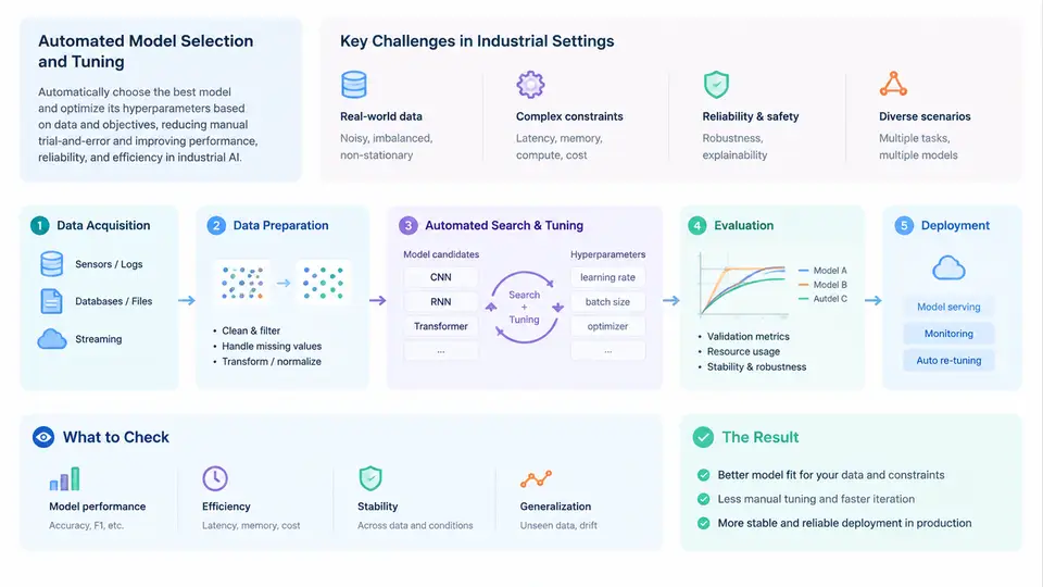
Industrial AI is not simply machine learning applied to factory data. It is a discipline defined by hard constraints: models must run on edge devices with limited compute, predictions must be traceable for quality audits, and a model that drifts silently can halt a production line. Within this landscape, automated model selection and tuning addresses a practical bottleneck — the manual effort of choosing an algorithm family and searching its hyperparameter space for every new asset, product variant, or sensor configuration.
Automated model selection (AMS) is the process of evaluating candidate algorithms and feature pipelines against a defined objective and selecting the best-performing configuration without exhaustive human trial. Automated tuning (often called hyperparameter optimization, HPO) is the search over a model's configuration space — learning rate, tree depth, regularization strength, window size — guided by a search strategy such as Bayesian optimization or successive halving. In industrial practice the two are coupled: selection decides which model class, tuning decides how well that class performs.
Why Industrial Settings Change the Problem
Three constraints distinguish industrial AI from benchmark-driven ML:
- Data scarcity and imbalance. A bearing may fail twice in three years. Fault classes are rare, so accuracy is misleading; precision-recall and cost-weighted metrics dominate.
- Non-stationarity. Tool wear, seasonal temperature, and raw-material batches shift the input distribution. A tuned model degrades without retraining triggers.
- Deployment constraints. A 200 ms inference budget on a PLC-adjacent edge gateway rules out large ensembles regardless of offline accuracy.
These constraints mean the search objective is rarely "maximize F1." It is a constrained optimization: maximize detection quality subject to latency, memory, and interpretability budgets.
The End-to-End Pipeline
The pipeline below is the backbone of every subsequent chapter. Each stage produces artifacts consumed by the next, and automation can be inserted at any stage.
Each stage has an automation surface. Acquisition can be scheduled and versioned; preprocessing can be parameterized as part of the search space; feature engineering can be automated via tsfresh or catch22; AMS/HPO is the core automation engine; deployment closes the loop with monitoring that feeds back into retraining.
A Concrete Example: Bearing Fault Detection
Consider a vibration-based bearing fault classifier on a motor test rig. The input is a 10 kHz accelerometer signal sampled in 1-second windows. The task is to classify {healthy, inner-race fault, outer-race fault}.
A practical AMS/HPO configuration might look like this:
search_space:
  model: [RandomForest, GradientBoosting, SVM_RBF, 1D_CNN]
  window_size_ms: [200, 500, 1000]
  feature_set: [time_domain, freq_domain, combined]
  n_estimators: [50, 200, 500]        # tree models only
  C: [0.1, 1, 10]                     # SVM only
  learning_rate: [1e-3, 1e-4]         # CNN only
objective:
  metric: pr_auc_macro
  constraints:
    inference_latency_ms: "<= 200"
    model_size_mb: "<= 5"
sampler: bayesian
pruner: median_stopping
budget: 60 trials
After 60 trials, suppose the search returns a GradientBoosting model with window_size_ms=500, feature_set=combined, and n_estimators=200, achieving a cross-validated macro PR-AUC of 0.91 at 38 ms inference latency. The 1D CNN reaches 0.93 PR-AUC but exceeds the latency budget at 240 ms, so it is rejected by the constraint filter — not by accuracy. This is the essential industrial lesson: the best model is the best feasible model.
Failure Modes to Anticipate
Two failure modes appear repeatedly in industrial AMS/HPO:
- Objective mismatch. Optimizing accuracy on a 98% healthy dataset selects a trivial majority-class predictor. Always verify the objective against a cost matrix or PR curve.
- Search space leakage. If preprocessing parameters (e.g., normalization statistics) are computed on the full dataset before splitting, the search overfits the validation fold. Fit scalers inside each CV fold.
Typical symptoms and checks: if validation PR-AUC is high but deployment performance collapses, suspect distribution shift between the training batch and the live line — compare feature histograms per shift. If the search converges to the same model every run regardless of seed, the search space is too narrow or the pruner is terminating trials prematurely.
What This Chapter Establishes
The pipeline above is the reference architecture for the rest of the course. Automated model selection and tuning sit at the center, but they are only useful when bounded by deployment constraints and fed by trustworthy data. The next chapters will open each stage: acquisition and labeling strategy, feature automation, search algorithms (Bayesian optimization, Hyperband, ASHA), multi-objective trade-offs, and deployment-time monitoring. The recurring principle is that automation must be constraint-aware — a search that ignores latency, memory, or label cost will produce models that never reach the factory floor.