1. Course overview
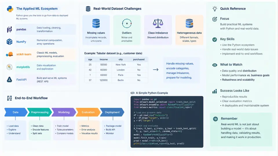
Machine learning courses often begin with an algorithm and end with a metric. Applied ML systems begin with a problem and end with a running service that someone depends on. The difference is not academic. A model that achieves 0.94 AUC on a held-out split but cannot be retrained when the data schema shifts, cannot explain a prediction to a compliance reviewer, or cannot survive a 3 a.m. traffic spike is not a system — it is an experiment. This chapter frames the entire course around that distinction and introduces the Python ecosystem and workflow patterns you will use in every subsequent chapter.
What Makes an ML System "Applied"
An applied ML system is a software system whose behavior is partly determined by a model learned from data. That definition implies four non-negotiable properties:
- Reproducibility — given the same code, data snapshot, and configuration, training produces the same artifact (within documented numerical tolerance).
- Observability — inputs, predictions, latency, and drift are logged and queryable after deployment.
- Maintainability — retraining, rollback, and schema evolution are routine operations, not emergencies.
- Accountability — every prediction can be traced to a model version, a feature set, and a decision threshold.
These properties are engineering concerns, not modeling concerns. Most production failures in ML are not caused by choosing the wrong algorithm; they are caused by training/serving skew, silent data corruption, unversioned feature logic, or a threshold that was tuned on a dataset that no longer resembles reality.
The Python Ecosystem: Layers, Not a Single Tool
Python's strength for applied ML is that it covers the entire pipeline with mature, interoperable libraries. It helps to think in layers rather than in a flat list of packages:
| Layer | Responsibility | Representative libraries |
|---|---|---|
| Data ingestion & storage | Read/write Parquet, CSV, SQL, object stores | pandas, polars, pyarrow, SQLAlchemy |
| Numerical & tabular compute | Array math, joins, group-by, window ops | numpy, pandas, scipy |
| Modeling | Classical ML, gradient boosting, deep learning | scikit-learn, xgboost, lightgbm, torch |
| Experiment tracking | Params, metrics, artifacts, lineage | mlflow, wandb |
| Serving | HTTP/gRPC inference, batching | FastAPI, BentoML, TorchServe |
| Orchestration | Scheduling, retries, dependency graphs | Airflow, Prefect, Dagster |
| Validation & monitoring | Schema checks, drift detection | pandera, great_expectations, evidently |
The practical rule: pick one library per layer, pin versions, and make the boundaries between layers explicit. A common anti-pattern is feature engineering logic written inline in a notebook, then re-implemented differently in the serving path. That duplication is the single most common source of training/serving skew.
Real-World Dataset Challenges
Textbook datasets are clean, balanced, stationary, and small. Real datasets are none of those things. The challenges you will encounter repeatedly fall into recognizable categories:
- Missingness with structure — values are not missing at random. A
credit_scorefield missing more often for rejected applicants encodes the rejection itself. - Leakage — a feature that would not be available at prediction time (e.g.,
account_closed_datewhen predicting churn) inflates offline metrics and collapses in production. - Class imbalance — fraud, failure, and conversion events are rare. Accuracy becomes meaningless; precision-recall and calibrated probabilities matter.
- Temporal drift — the joint distribution P(X, y) changes over time. A random train/test split leaks future information into the past.
- Schema and unit drift — a column changes from dollars to cents, or a categorical value is renamed upstream, silently degrading the model.
- Label noise and delay — ground truth arrives weeks later, or is itself a proxy for the outcome you actually care about.
The End-to-End Workflow
The workflow below is the backbone of this course. It is iterative, not linear: monitoring results feed back into data collection, which feeds back into feature design.
Each stage has a concrete deliverable and a concrete failure mode. Stage 1 produces a written problem statement with a target variable, a prediction time, and a decision the prediction will inform. Stage 2 produces a data audit: row counts, missingness rates, cardinality, and a documented time range. Stage 3 produces a feature pipeline that can be executed identically in training and serving. Stage 4 produces a model artifact plus an evaluation report sliced by time, segment, and threshold. Stage 5 produces a versioned endpoint with input validation. Stage 6 produces dashboards and alerts that trigger the feedback loops shown in orange.
A Minimal Reproducible Skeleton
The following skeleton is the pattern you will extend throughout the course. It is deliberately small, but it already enforces reproducibility and time-based splitting — two properties that most tutorials omit.
# train.py — reproducible baseline
import pandas as pd
from sklearn.model_selection import TimeSeriesSplit
from sklearn.ensemble import GradientBoostingClassifier
from sklearn.metrics import roc_auc_score, average_precision_score
import mlflow

DATA = "data/events.parquet"
TARGET = "converted"
TIME_COL = "event_ts"

df = pd.read_parquet(DATA).sort_values(TIME_COL)
X = df.drop(columns=[TARGET, TIME_COL])
y = df[TARGET]

splitter = TimeSeriesSplit(n_splits=5)
scores = []
with mlflow.start_run():
    mlflow.log_param("n_estimators", 300)
    for fold, (tr, te) in enumerate(splitter.split(X)):
        model = GradientBoostingClassifier(n_estimators=300, random_state=0)
        model.fit(X.iloc[tr], y.iloc[tr])
        p = model.predict_proba(X.iloc[te])[:, 1]
        scores.append({
            "fold": fold,
            "auc": roc_auc_score(y.iloc[te], p),
            "ap": average_precision_score(y.iloc[te], p),
        })
    mlflow.log_metrics({k: sum(s[k] for s in scores)/len(scores)
                        for k in ("auc", "ap")})
print(pd.DataFrame(scores))
Run this and you get per-fold AUC and average precision, plus a logged run in MLflow. If AUC varies wildly across folds, that is temporal drift, not model instability — and it is exactly the signal that a random split would have hidden. Typical failure symptoms at this stage: KeyError on a renamed column (schema drift), AUC near 0.99 on the first fold (leakage), or NaN in the feature matrix (missingness not handled). Each has a distinct diagnostic path, and we will cover them in later chapters.
What You Will Build
By the end of this course you will have built a complete applied ML system on a real, messy dataset: a data audit and validation layer, a versioned feature pipeline, a trained and evaluated model with calibrated probabilities, a FastAPI inference service with input schema validation, and a monitoring dashboard that detects drift and triggers retraining. Every chapter adds one production-grade component to that system, and every component is tested against the same dataset so you can see how the pieces interact.
The mindset to carry forward is simple: treat the model as one component among many, treat the data contract as the most important interface, and treat monitoring as the beginning of the next iteration rather than the end of the project.