1. Industrial equipment monitoring landscap
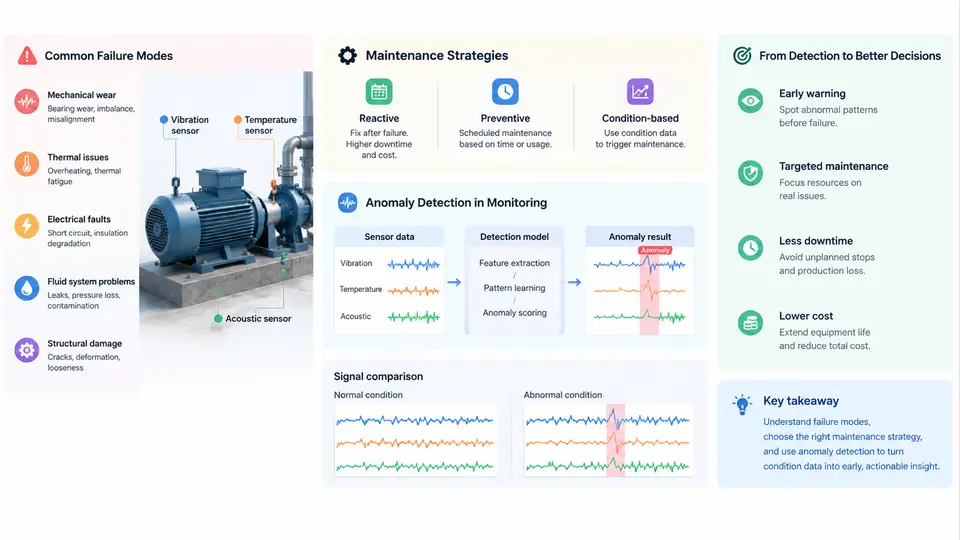
Industrial equipment monitoring sits at the intersection of reliability engineering, control systems, and data science. Before any anomaly detection model is trained or any threshold is tuned, an engineer must understand what can go wrong with a machine, how maintenance decisions are currently made, and where automated detection fits into that decision loop. This chapter establishes that foundation by walking through the physical failure mechanisms that generate detectable signals, the evolution of maintenance strategies from reactive to predictive, and the specific position anomaly detection occupies within condition-based maintenance (CBM).
Failure Modes: The Physical Sources of Anomalous Signals
Every anomaly detection system ultimately traces back to a physical degradation process. A failure mode is the specific manner in which a component ceases to perform its intended function. For rotating machinery — pumps, motors, compressors, fans, gearboxes — the dominant failure modes are well catalogued, and each produces a characteristic signature in vibration, temperature, current, or acoustic emissions.
Consider a centrifugal pump driven by an induction motor through a rolling-element bearing. Common failure modes include:
- Bearing spalling and fatigue: Repeated rolling contact stress causes subsurface cracks that propagate to the raceway surface. The resulting impacts generate high-frequency vibration bursts at characteristic defect frequencies (BPFO, BPFI, FTF, BSF). Early-stage spalling may be invisible in overall vibration RMS but clearly visible in envelope-demodulated spectra.
- Imbalance: Mass eccentricity produces a once-per-revolution (1×) radial force. Vibration amplitude at 1× running speed increases proportionally to the imbalance magnitude. Phase remains stable relative to a keyphasor reference.
- Misalignment: Shaft centerline offset or angularity between driver and driven equipment generates strong 2× and sometimes 3× harmonics, often with axial vibration components. Unlike imbalance, the 1× component may not dominate.
- Cavitation: Local pressure drops below vapor pressure, causing vapor bubble formation and collapse. This produces broadband high-frequency noise, often described as "gravel" or "popping," and can erode impeller surfaces rapidly.
- Seal wear and leakage: Mechanical seal face degradation increases leakage flow and can alter axial thrust, indirectly changing vibration and temperature patterns.
Each failure mode has a progression timeline. Some, like bearing fatigue, evolve over weeks to months and offer ample warning. Others, like cavitation-induced erosion or sudden seal failure, can escalate within hours. The detection system's sampling rate, feature set, and alarm thresholds must be matched to the fastest failure mode of concern.
Maintenance Strategies: From Reactive to Predictive
Maintenance strategy determines how and when intervention occurs. The four canonical strategies form a spectrum of increasing sophistication and cost:
| Strategy | Trigger | Typical Cost Profile | Limitation |
|---|---|---|---|
| Reactive (run-to-failure) | Equipment stops working | Low planned cost, high unplanned cost | Secondary damage, safety risk, production loss |
| Preventive (time-based) | Calendar or runtime interval | Moderate, predictable | Over-maintenance of healthy assets, under-maintenance of fast-wearing ones |
| Condition-based (CBM) | Measured condition indicator crosses threshold | Moderate, optimized by actual state | Requires sensors, baselines, and threshold logic |
| Predictive (PdM) | Forecast of remaining useful life (RUL) | Higher upfront, lowest total lifecycle | Needs historical failure data and degradation models |
In practice, most plants operate a hybrid. Safety-critical or inaccessible equipment (subsea pumps, turbine generators) justifies predictive strategies. Non-critical, cheap-to-replace items (small fans, light-duty conveyors) may remain reactive. The economic decision hinges on the ratio of unplanned downtime cost to monitoring implementation cost.
Where Anomaly Detection Fits in Condition-Based Maintenance
Condition-based maintenance relies on a decision rule: if a condition indicator exceeds a threshold, trigger maintenance. The simplest CBM uses fixed thresholds — for example, ISO 10816 vibration severity zones for industrial machines. But fixed thresholds suffer from two problems: they are machine-specific and operating-point-specific, and they cannot detect novel or slowly developing anomalies that never cross a static limit.
Anomaly detection addresses both gaps. Instead of asking "Is vibration above 4.5 mm/s RMS?", it asks "Does the current multivariate pattern of vibration, temperature, current, and pressure deviate from the learned normal behavior of this specific machine under these specific operating conditions?" This shift from absolute limits to relative deviation enables earlier detection and fewer false alarms across varying loads and speeds.
The integration point is the CBM decision loop. An anomaly detector outputs a score or label. That output feeds a maintenance decision logic that considers criticality, production schedule, and spare parts availability. The detector does not make the maintenance decision; it informs it.
Key distinction: Anomaly detection identifies deviation from normal. Fault diagnosis identifies which fault is present. Prognostics estimates how long until functional failure. A complete CBM system may use all three, but anomaly detection is typically the first layer because it requires only normal data for training — a critical advantage when failure examples are scarce.
From Signal to Decision: A Concrete Example
To make the landscape concrete, consider a 75 kW centrifugal pump on a cooling water loop. The monitoring system collects triaxial vibration at the drive-end bearing, motor current, discharge pressure, and bearing temperature at 1 Hz for temperature and pressure, and 25.6 kHz for vibration bursts.
During commissioning, the pump runs across its normal operating envelope: flow varies from 60% to 100% of design, ambient temperature from 15°C to 35°C. A baseline model learns the joint distribution of features — 1× amplitude, 2× amplitude, high-frequency envelope RMS, temperature rise above ambient, and current harmonic distortion — as a function of flow rate and ambient temperature.
Six weeks later, the high-frequency envelope RMS at the drive-end bearing begins a slow upward trend. At the same flow rate and ambient temperature, the envelope RMS is 2.3 standard deviations above the baseline mean. The 1× amplitude remains normal. Temperature rises by 1.8°C. The anomaly detector flags a deviation. A vibration analyst reviews the envelope spectrum and finds early BPFO harmonics. Maintenance is scheduled during the next planned outage, and the bearing is replaced before spalling reaches the raceway surface.
This example illustrates the core value proposition: detection occurs weeks before a fixed threshold would trigger, and the maintenance action is planned rather than reactive.
Practical Implications for System Design
Three design principles follow from this landscape view. First, sensor selection must match failure modes. A bearing fault detector needs high-frequency vibration or acoustic emission; a thermal fault detector needs temperature and current. Deploying the wrong sensor modality guarantees missed detections regardless of algorithm quality.
Second, baseline learning must cover the operating envelope. A model trained only at 100% flow will false-alarm at 60% flow. The training data must span the normal range of load, speed, ambient conditions, and product changes.
Third, anomaly detection is a layer, not a solution. It must connect to maintenance decision logic that weighs criticality and logistics. A detection without a response path is just a data point.
Practical starting point: For a first CBM deployment, select 3–5 critical rotating machines with known failure history. Instrument them with triaxial vibration and temperature. Collect 4–6 weeks of baseline data across normal operating conditions. Implement a simple multivariate anomaly detector (e.g., Mahalanobis distance or autoencoder reconstruction error). Validate against any known historical failures before trusting live alarms.
The remaining chapters build on this foundation: signal processing for feature extraction, statistical and machine learning detectors, alarm management, and integration with computerized maintenance management systems (CMMS). Each layer assumes the landscape described here — physical failure modes generating signals, maintenance strategies defining the decision context, and anomaly detection occupying the detection layer between sensing and action.