📚 Course ContentsChapter 1 Course overview

1. Course overview

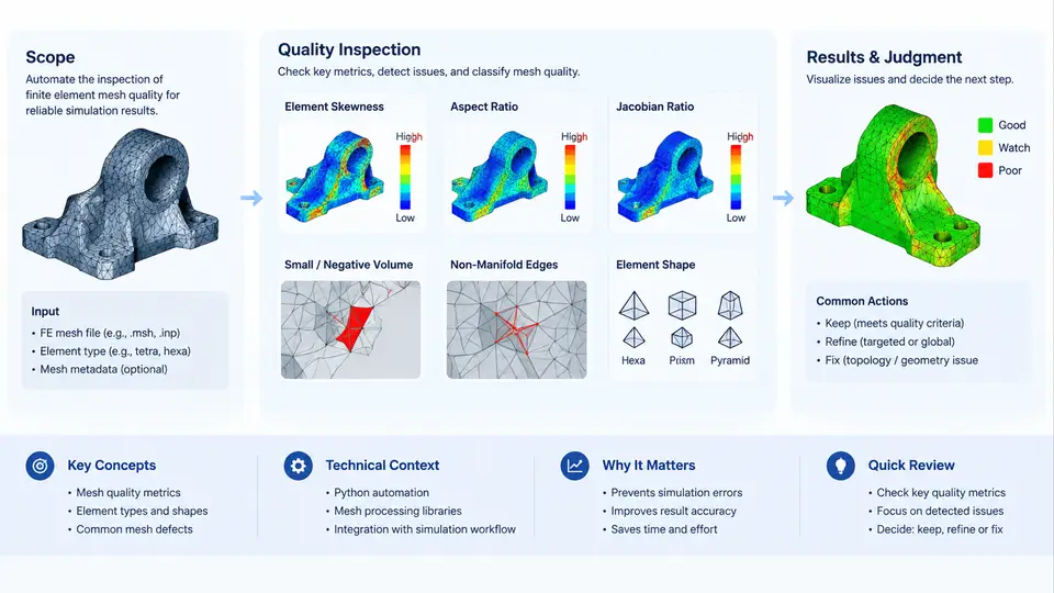
Finite element analysis (FEA) is only as trustworthy as the mesh it runs on. A solver will happily return a displacement field, a stress contour, or a modal frequency from a mesh full of sliver elements and negative Jacobians — and those numbers can be confidently wrong. Mesh quality inspection is the discipline of catching those defects before they contaminate results. Mesh quality inspection automation is the practice of encoding that discipline into reproducible Python programs that read a mesh, compute quality metrics, apply acceptance criteria, and produce actionable reports without manual clicking through a GUI.

This course targets that automation layer. It assumes you already understand what a finite element mesh is and are comfortable with basic Python. Over 30 chapters we move from metric definitions and file formats, through vectorized NumPy implementations and threshold logic, to CI integration, regression baselines, and repair-triggering workflows. The goal is not to replace your mesher — it is to build a quality gate that runs the same way on your laptop, in a batch job, and in a pipeline.

Why automate mesh checking at all?

Manual inspection does not scale. A single component may contain 200,000 elements; a full vehicle model tens of millions. Even when a GUI highlights "bad" elements, the criteria are often implicit, applied inconsistently between engineers, and impossible to audit six months later. Automation addresses three concrete failures:

Inconsistency. Two engineers checking the same mesh against "aspect ratio < 5" may disagree on whether a warped quad counts. A script does not.
Late detection. A bad mesh discovered after a 14-hour solve wastes the solve. A pre-solve gate rejects it in seconds.
No traceability. When a result is questioned, you need the exact metric values and thresholds that were applied. A generated report provides that evidence.

The economic argument is straightforward: inspection cost scales with mesh size linearly, while the cost of a wrong result scales with the consequences of the decision it informs.

Core concepts and vocabulary

Before writing code, fix the vocabulary. A quality metric is a scalar function of element geometry — for example, the Jacobian ratio, aspect ratio, skew, or warpage of a single element. A threshold is the acceptance boundary for that metric. A criterion combines a metric, a threshold, and a comparison direction (e.g., jacobian_ratio >= 0.3). A violation is an element that fails at least one criterion. A quality gate is the decision rule that converts violations into a pass/fail verdict for the whole mesh.

Two distinctions matter throughout the course. First, element-type dependence: a metric meaningful for a hexahedron (e.g., Jacobian ratio) may be undefined or differently defined for a tetrahedron or shell. Second, normalization: some metrics are dimensionless ratios in [0, 1], others are absolute lengths or angles. Mixing them without normalization makes threshold tables unreadable and error-prone.

Convention used in this course: all normalized metrics are reported so that 1.0 is ideal and 0.0 is degenerate. Where a metric is naturally "lower is better" (e.g., aspect ratio), we state the raw definition explicitly and never silently invert it. Any figure or table will label the direction.

The inspection pipeline

Every automated checker, regardless of mesher or solver, follows the same logical pipeline. Understanding it as a data flow — not a list of steps — is what lets you swap components later.

The pipeline is deliberately linear in its data flow but not in its control flow. The dashed feedback path is where automation earns its keep: a failing verdict can trigger a local remesh, a mesh-smoothing pass, or simply a ticket. Whether you close that loop is a policy decision, but the architecture should make it possible.

What "automation" actually means here

Automation in this course means four concrete capabilities, each testable:

Headless execution. The checker runs from a command line or CI runner with no GUI, no license checkout for a pre-processor, and deterministic output.
Declarative criteria. Thresholds live in a config file (YAML/JSON), not in code. Changing a limit does not require editing a script.
Structured output. Results are machine-readable (CSV/JSON) plus a human-readable summary, so both dashboards and engineers can consume them.
Reproducibility. Given the same mesh and config, the checker produces byte-identical verdicts. This is what makes regression testing possible.

A useful mental model: the checker is a compiler for mesh quality. The mesh is source code, the criteria set is the language specification, and the verdict is the compile result. Just as you would not ship code that fails to compile, you should not ship a mesh that fails its quality gate.

A minimal worked example

To make the scope concrete, consider a small tetrahedral mesh stored as a node array and a connectivity array. The following snippet computes a normalized Jacobian ratio for each tet and flags violations. It is illustrative, not production code — production versions handle degenerate cases, vectorize across millions of elements, and support multiple element types.

import numpy as np

# nodes: (N, 3) float array; tets: (M, 4) int array of node indices
def tet_jacobian_ratio(nodes, tets):
    p0, p1, p2, p3 = (nodes[tets[:, i]] for i in range(4))
    # edge vectors from p0
    e1, e2, e3 = p1 - p0, p2 - p0, p3 - p0
    # signed volume via scalar triple product
    vol6 = np.einsum('ij,ij->i', np.cross(e1, e2), e3)
    # ideal reference volume for a regular tet of the same edge scale
    # (simplified: use max edge length as characteristic length)
    edges = np.stack([np.linalg.norm(e1, axis=1),
                      np.linalg.norm(e2, axis=1),
                      np.linalg.norm(e3, axis=1)], axis=1)
    h = edges.max(axis=1)
    ideal = h**3 / (6.0 * np.sqrt(2.0))
    ratio = np.abs(vol6) / 6.0 / ideal
    return np.clip(ratio, 0.0, 1.0)

# Example: flag elements below 0.3
ratio = tet_jacobian_ratio(nodes, tets)
violations = np.where(ratio < 0.3)[0]
print(f"{len(violations)} of {len(tets)} elements below threshold")

Run this on a mesh with a known sliver and you will see the violation count jump. That immediate, quantitative feedback — element IDs, metric values, threshold — is the entire point of the course. Everything that follows is about making this snippet robust, fast, configurable, and integrated.

Technical context and boundaries

This course is mesher-agnostic and solver-agnostic. We read common formats (Gmsh .msh, Abaqus .inp, Nastran .bdf) and compute metrics from first principles, so the techniques transfer whether you use CalculiX, Code_Aster, Ansys, or a custom solver. We do not cover mesh generation algorithms, CAD healing, or solver convergence debugging except where they intersect the quality gate.

Scope boundary: A passing quality gate does not guarantee an accurate solution. It guarantees the mesh is free of the geometric defects that most commonly cause solver errors or silent inaccuracy. Mesh convergence and physics validation remain separate, necessary activities.

What you will be able to do

By the end of the course you will be able to: define and justify a criteria set for a given element type and analysis type; implement vectorized metric computations in NumPy; parse and normalize at least three mesh file formats; build a configurable, headless checker with structured output; integrate it into a CI pipeline with regression baselines; and design a repair-triggering workflow that closes the loop from verdict back to mesh. Each chapter builds one component of that system, and the final chapters assemble them into a reusable package.

The next chapter begins with the metric definitions themselves — what each quality measure actually computes, and why the choice of metric determines what defects your gate can and cannot catch.