3. 迭代反投影超分辨率
任务说明
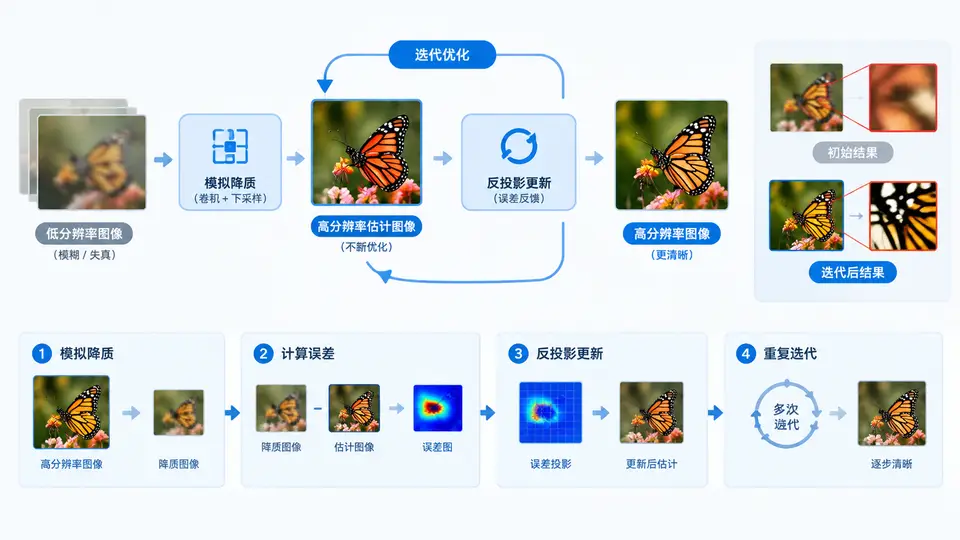
本案例实现经典的迭代反投影(Iterative Back-Projection, IBP)超分辨率算法。给定一张低分辨率输入图像,通过模拟“高分辨率图像→降质→低分辨率图像”的成像过程,迭代修正当前高分辨率估计,使模拟降质结果逼近真实低分辨率输入,从而重建出细节更丰富的高分辨率图像。
算法原理与实现
IBP的核心思想是:设当前高分辨率估计为 X,降质模型为 H(包含模糊与下采样),真实低分辨率图像为 Y。每次迭代计算残差 Y - H(X),将该残差通过反向投影算子 H^T 映射回高分辨率网格并累加到 X 上,即 X ← X + H^T(Y - H(X))。本实现采用双三次插值作为降质模型中的下采样操作,反向投影使用双三次插值的转置近似(即对残差上采样后与高斯核卷积)。
代码实现
import numpy as np
from scipy.ndimage import gaussian_filter, zoom
from skimage import io, color
import matplotlib.pyplot as plt

def im2double(img):
    """转换为float64且范围[0,1]"""
    if img.dtype == np.uint8:
        return img.astype(np.float64) / 255.0
    return img.astype(np.float64)

def degrade(img_hr, scale=4, sigma=1.5):
    """模拟降质:高斯模糊 + 下采样"""
    img_blur = gaussian_filter(img_hr, sigma=sigma)
    h, w = img_blur.shape[:2]
    h_lr, w_lr = h // scale, w // scale
    # 使用zoom进行下采样(双三次)
    img_lr = zoom(img_blur, (1/scale, 1/scale) + (1,)*(img_hr.ndim-2), order=3)
    return img_lr

def back_project(residual_lr, scale=4, sigma=1.5):
    """反向投影:残差上采样 + 高斯平滑"""
    # 上采样到高分辨率尺寸
    h_lr, w_lr = residual_lr.shape[:2]
    h_hr, w_hr = h_lr * scale, w_lr * scale
    up = zoom(residual_lr, (scale, scale) + (1,)*(residual_lr.ndim-2), order=3)
    # 平滑作为转置模糊的近似
    up_smooth = gaussian_filter(up, sigma=sigma)
    return up_smooth

def ibp_super_resolution(img_lr, scale=4, iterations=30, lr=0.5, sigma=1.5):
    """
    迭代反投影超分辨率
    参数:
        img_lr: 低分辨率图像 (H, W) 或 (H, W, C),float64 [0,1]
        scale: 放大倍数
        iterations: 迭代次数
        lr: 更新步长
        sigma: 高斯核标准差
    返回:
        img_hr: 高分辨率估计
    """
    # 初始化:双三次插值放大
    h_lr, w_lr = img_lr.shape[:2]
    h_hr, w_hr = h_lr * scale, w_lr * scale
    img_hr = zoom(img_lr, (scale, scale) + (1,)*(img_lr.ndim-2), order=3)

    for it in range(iterations):
        # 模拟降质
        img_degraded = degrade(img_hr, scale, sigma)
        # 计算残差(低分辨率空间)
        residual = img_lr - img_degraded
        # 反向投影到高分辨率空间
        correction = back_project(residual, scale, sigma)
        # 更新
        img_hr = img_hr + lr * correction
        # 裁剪到有效范围
        img_hr = np.clip(img_hr, 0, 1)

    return img_hr

# ========== 主程序示例 ==========
if __name__ == "__main__":
    # 生成测试图像(使用内置示例或合成图像)
    # 这里使用skimage的astronaut图像并手动降质来验证
    try:
        img_ref = io.imread('https://scikit-image.org/_static/img/logo.png', as_gray=True)
        # 若网络不可用则使用合成图像
        if img_ref is None:
            raise ValueError()
    except:
        # 合成测试图:包含高频细节的棋盘+圆
        y, x = np.mgrid[0:128, 0:128]
        img_ref = 0.5 + 0.3*np.sin(x/3.0)*np.cos(y/3.0)
        img_ref += 0.2*((x//8 + y//8) % 2)  # 棋盘格

    img_ref = im2double(img_ref)
    # 模拟低分辨率观测
    img_lr = degrade(img_ref, scale=4, sigma=1.5)

    # 执行IBP重建
    img_hr_ibp = ibp_super_resolution(img_lr, scale=4, iterations=30)

    # 对比:直接双三次插值
    img_bicubic = zoom(img_lr, 4, order=3)

    # 计算PSNR(以原始高分辨率图为参考)
    def psnr(img1, img2):
        mse = np.mean((img1 - img2)**2)
        if mse == 0:
            return float('inf')
        return 10 * np.log10(1.0 / mse)

    psnr_bicubic = psnr(img_ref, img_bicubic)
    psnr_ibp = psnr(img_ref, img_hr_ibp)

    print(f"双三次插值 PSNR: {psnr_bicubic:.2f} dB")
    print(f"IBP重建 PSNR: {psnr_ibp:.2f} dB")

    # 保存结果
    plt.figure(figsize=(12,4))
    plt.subplot(1,3,1); plt.imshow(img_lr, cmap='gray'); plt.title('低分辨率输入')
    plt.subplot(1,3,2); plt.imshow(img_bicubic, cmap='gray'); plt.title('双三次插值')
    plt.subplot(1,3,3); plt.imshow(img_hr_ibp, cmap='gray'); plt.title('IBP重建')
    plt.tight_layout()
    plt.savefig('ibp_result.png', dpi=150)
    plt.close()
运行与验证
依赖安装:
pip install numpy scipy scikit-image matplotlib运行方式:将上述代码保存为 ibp_sr.py,在终端执行 python ibp_sr.py。
验证方法:程序会输出双三次插值与IBP重建的PSNR值,并保存对比图 ibp_result.png。判定标准:IBP的PSNR应高于双三次插值(通常高1~3dB),且重建图像边缘更锐利、振铃伪影更少。若使用合成图像,由于降质模型与算法假设完全一致,IBP应显著优于直接插值。
关键参数说明
| 参数 | 默认值 | 作用 |
|---|---|---|
| scale | 4 | 超分辨率放大倍数 |
| iterations | 30 | 迭代次数,越多收敛越充分 |
| lr (λ) | 0.5 | 更新步长,过大震荡,过小收敛慢 |
| sigma | 1.5 | 降质模型高斯核标准差,需与真实模糊匹配 |
判定标准:当迭代过程中残差能量 ||Y - H(X)||² 持续下降并趋于平稳时,说明算法收敛。若PSNR相比双三次插值提升超过0.5dB,且视觉上边缘更清晰、无新增伪影,即可判定实现正确。